Simulate correlated continuous and discrete variables

Statistical software provides methods to simulate independent random variates from continuous and discrete distributions. For example, in the SAS DATA step, you can use the RAND function to simulate variates from continuous distributions (such as the normal or lognormal distributions) or from discrete distributions (such as the Bernoulli or Poisson). The resulting variables are uncorrelated. Depending on your situation, this may or may not be acceptable.

My book, Simulating Data with SAS (Wicklin, 2013), devotes two chapter (Ch. 8 and 9) to simulating correlated multivariate data, both continuous and discrete. Some of the techniques are complicated and require using sophisticated SAS IML programs. However, my recent blog post about polychoric correlation suggests a relatively simple way to specify the correlations between an arbitrary number of continuous and discrete variates. This article shows how to simulate data from a multivariate normal distribution, then bin some of the variables to obtain ordinal variables that are correlated with each other and with the continuous variables. The method requires using only two procedures: the SAS DATA step and PROC SIMNORMAL in SAS/STAT software.

Simulate uncorrelated data in the DATA step

As mentioned earlier, it is straightforward to simulate uncorrelated data by using the SAS DATA step. For example, the following DATA step simulates two continuous variables (X1 and X2) and two discrete variables, A and B. The A variable contains two levels (1 and 2), and the B variable contains three levels (1, 2, and 3). The discrete variables are generated by using the "TABLE" distribution, which enables you to specify the number of levels and the probability for each level. In the following DATA step, the value A=1 is generated with probability 2/3, and the value A=2 is generated with probability 1/3. Similarly, P(B=1) = 0.5, P(B=2) = 0.3, and P(B=3) = 0.2.

/* generate random variates independently */
%let n = 5000;
data UncorrMV;
call streaminit(12345);
do i = 1 to &n;
   x1 = rand("Normal", 0, 1);          /* x1 ~ N(0,1) */
   x2 = rand("Normal", 0, 1);          /* x2 ~ N(0,1) */
   A  = rand("Table", 2/3, 1/3);       /* P(A=1)=2/3; P(A=2)=1/3 */
   B  = rand("Table", 0.5, 0.3, 0.2);  /* P(B=1)=0.5; P(B=2)=0.3; P(B=3)=0.2 */
   output;
end;
run;
 
/* show that x1 and x2 are uncorrelated */
proc corr data=UncorrMV nosimple;
   var x1 x2;
run;
/* show that A and B are not associated */
proc corr data=UncorrMV nosimple polychoric;
   var A B;
run;

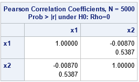
The output from the first call to PROC CORR is shown. It shows that the sample correlation between x1 and x2 is -0.009. The p-value (0.54) is large, which implies that the correlation is not significantly different from 0. Similarly, the output from the second call to PROC CORR (not shown) shows that the sample polychoric correlation between A and B is not significantly different from 0.

The remainder of this article shows how to modify the simulation to obtain correlations between all variables.

The multivariate normal distribution

Statistical software supports simulating multivariate normal random variates by specifying a mean vector and a covariance matrix. If you specify a correlation matrix (instead of a general covariance matrix) you can easily generate, say, four correlated variables. Specify a mean of zero for the variable that are to be binned, so that they are distributed as N(0, 1).

As shown in a previous article you can bin a standard normal variable to obtain a categorical variable. The endpoints of the bins (called cut points) determine the relative proportion of the levels for the categories. For example, suppose you want to create a categorical variable, A, from a standard normal variable, X. If you want A to have two equally likely categories, you can use x=0 as a cut point because P(X < 0) = P(X > 0) = 1/2. If you want unequal proportions, you can use the quantile function of the standard normal distribution to determine the cut points. For example, if you want P(A=1) = 2/3, you can set the cut point x=0.43 because Φ(0.43) ≈ 2/3, where Φ is the standard normal cumulative distribution function (CDF).

This suggests a simple algorithm: Simulate several correlated normal variables, then bin some of them to produce categorical variables.

In SAS, recall that you can use PROC SIMNORMAL to simulate from the multivariate normal distribution. The following DATA step creates a special SAS data set that contains the mean vector and covariance matrix for a four-variable multivariate normal distribution. That data set is read by the SIMNORMAL procedure, which then generates random variates from the distribution:

/* Create a TYPE=COV data set that specifies mean and covariance parameters 
   In this example, the COV matrix is actually a correlation matrix. */
data MyCov(type=COV);
input _TYPE_ $ 1-8 _NAME_ $ 9-16 x1 x2 y1 y2;
/*               x1  x2    y1  y2 */
datalines;
COV     x1       1   0.5  -0.2  0
COV     x2       0.5 1     0.1  0.4
COV     y1      -0.2 0.1   1   -0.4
COV     y2       0   0.4  -0.4  1
MEAN             5   10    0    0
;
 
/* generate random observations from the MVN distribution with 
   the specified mean and covariance */
proc simnormal data=MyCov outsim=MVN seed = 12345 /* random number seed */
               nr = &n;                           /* size of sample */
   var x1 x2 y1 y2;
run;
 
/* show that the sample correlations are close to the parameter values */
proc corr data=MVN nosimple;
   var x1 x2 y1 y2;
run;

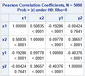
The following list shows the parameter values. The output from PROC CORR shows that the sample estimates for the simulated data are very close to the distribution parameters.

The correlation between X1 and X2 is 0.5. The sample estimate is 0.51.
The correlation between Y1 and Y2 is -0.4. The sample estimate is 0.404.
There are also correlations between the X and Y variables: corr(X1, Y1) = -0.2, corr(X2, Y1) = 0.1, corr(X1, Y2) = 0, and corr(X2, Y2) = 0.4. The sample estimates are close to the parameter values. Notice that the p-value is large for the X1 and Y2 sample, which indicates the variables are uncorrelated.

Create ordinal variables by binning normal variables

For this example, let's create ordinal variables, A and B, from Y1 and Y2. The variable A will have two levels and P(A=1) = 2/3. The variable A will have three levels and P(B=1) = 0.5 and P(B=2) = 0.3. The following DATA step bins the Y1 and Y2 variables to create A and B:

/* Use cut points (cp) to bin the MVN data into discrete ordinal variables.
   Use the quantile function to choose cut points for the 
   standard normal N(0,1) variables Y1 and Y2.
   Goal for A: P(A=1)=2/3; P(A=2)=1/3
   Goal for B: P(B=1)=0.5; P(B=2)=0.3; P(B=3)=0.2  
*/
data CorrVars;
   array cpA[1] _temporary_ (0.43);    /* A will have dim+1 = 2 levels */
   array cpB[2] _temporary_ (0 0.84);  /* B will have dim+1 = 3 levels */
   set MVN;
   A = 1;                              /* default category */
   do i = 1 to dim(cpA);               /* find the bin for y1; assign that number to A */
      if y1 > cpA[i] then 
         A = i+1;
   end;
   B = 1;                              /* default category */
   do i = 1 to dim(cpB);               /* find the bin for y2; assign that number to B */
      if y2 > cpB[i] then 
         B = i+1;
   end;
   output;
   drop i;
run;
 
/* We now have correlated continuous variables, correlated ordinal 
   variables, and correlation between the continuous and the ordinal variables
*/
proc corr data=CorrVars nosimple Polychoric;
   var A B;
run;
proc corr data=CorrVars nosimple Polyserial;
   var x1 x2;
   with A B;
run;

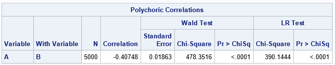
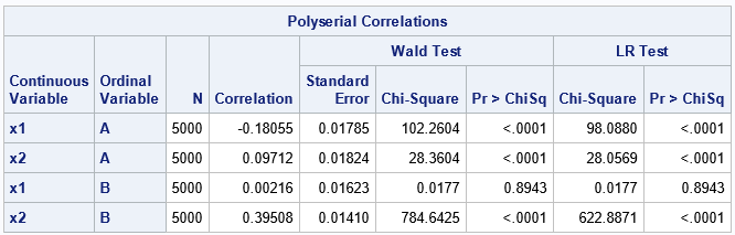
The binning process does not perfectly preserve the correlation estimates. Recall that the sample correlation for Y1 and Y2 is -0.404. After binning the Y1 and Y2 variables, the estimated polychoric correlation between A and B is -0.408. Similarly, recall sample correlation for X1 and Y1 is -0.193. After binning the Y1 variable, we estimate the polyserial correlations (which is an association between a continuous and a discrete variable) to be -0.181. Similar results hold for the other polyserial correlation estimates.

By using cut points to discretize the Y1 and Y2 variables, we have created ordinal variables, A and B, that are correlated with each other and with the continuous variables. Although the multivariate normal correlations are not preserved, the resulting polychoric and polyserial correlation estimates tend to be close to the estimates for the continuous variables.

Drawbacks of the multivariate normal technique

This simulation technique has an obvious drawback: it relies on the multivariate normal distribution. Not every variable is normally distributed. Not every discrete variable is obtained by binning a latent normal variable. Nevertheless, this method can be useful to simulate synthetic correlated data that you can use in examples or as one part of a simulation study.

Summary

This article presents a relatively simple way to simulate correlated data for examples or for simulation studies. You first simulate multivariate normal variates with a known correlation. You then bin some of the variables to obtain ordinal categorical variables. You can do this in a way that enables you to specify the relative proportions of the categories. The resulting categorical variables are correlated with the continuous variables and with the other categorical variables. The polyserial and polychoric estimates tend to be close to the original correlations in the multivariate normal distribution. The degree of "closeness" depends on the sample size. This article used Monte Carol samples with n=5,000 observations, which often results in 2-3 digits of accuracy.

This article shows how to perform these computations in SAS by using the DATA step and PROC SIMNORMAL in SAS. You can also perform the computations by using SAS IML software.

Blogs