SAS provides many built-in routines for data analysis. A previous article discusses polychoric correlation, which is a measure of association between two ordinal variables. In SAS, you can use PROC FREQ or PROC CORR to estimate the polychoric correlation, its standard error, and confidence intervals.
Although SAS provides a built-in method for estimating polychoric correlation, it is instructive to program the estimation algorithm from first principles. There are several reasons for doing this:
- Understand the statistic better: Programming the algorithm leads to a better understanding of polychoric correlation.
- Build programming skills: Although SAS provides an easy way to estimate the polychoric correlation, programming an algorithm builds skills and experience that can be used to compute statistics that SAS does not provide. For example, a SAS user asked whether SAS provides a way to estimate the polychoric correlation for weighted data. The answer is no, but if we know how to program the unweighted statistic, it might be possible to modify the algorithm to estimate the weighted statistic.
- Demonstrate the power of IML: In SAS, you can solve simple MLEs by using either the SAS IML language or PROC NLMIXED. Sometimes the likelihood function is very complicated and requires intermediate computations, such as solving integrals, estimating probabilities, and performing other computations. In these cases, the computational power and flexibility of the SAS IML language provide a clear advantage over PROC NLMIXED.
There is also a fourth reason: It's fun to program and learn new things! This article implements the MLE for the polychoric correlation as presented in Olsson (1979), "Maximum likelihood estimation of the polychoric correlation coefficient." The complete SAS program that creates all graphs and tables in this article is available from GitHub.
How to estimate polychoric correlation by using MLE
A previous article discusses polychoric correlation and the assumption that the ordinal variables are defined from latent bivariate normal (BVN) variables. The polychoric correlation is an estimate of the correlation of the underlying BVN variables and requires estimating the cut points that define the ordinal variables. This article shows how to perform the following steps. The statistical details are discussed in Olsson (1979):
- Define the example data. Use PROC FREQ to write the frequencies and marginal frequencies to data sets.
- Use PROC IML to read the frequencies. Estimate the thresholds (cut points) for the latent variables from the observed cumulative frequencies.
- For any correlation, ρ, compute the standard bivariate normal (BVN) probability for the rectangular regions defined by the thresholds.
- Define the log-likelihood function as a weighted sum that involves the observed frequencies and the BVN probabilities. Plot the log-likelihood as a function of the correlation, ρ.
- Use one-parameter MLE to estimate the polychoric correlation for the specified values of the threshold parameters (Olsson, p. 448).
- Use the preceding estimate as the initial guess for optimizing a log-likelihood function in which the threshold parameters are permitted to vary. This optimization provides the final estimate of polychoric correlation (Olsson, p. 447) and estimates for the threshold parameters.
Compute frequencies and marginal frequencies
Assume we have N observations and two ordinal variables, Y1 and Y2. The Y1 variable has k1 levels; the Y2 variables has k2 levels. You can display the joint distribution of frequency counts by using PROC FREQ. The FREQ procedure also enables you to display the cumulative percentages (or proportions) for each variable. For example, the following SAS code reproduces the data that were analyzed in a previous article, but renames the variables Y1 and Y2. The call to PROC FREQ writes the joint frequencies to a data set, and writes the marginal cumulative frequencies to separate data sets:
/* Encode the ordinal variables as 1,2,...,k. Use a SAS format to display the class levels. */ proc format; value QualFmt 1="Strongly Disagree" 2="Disagree" 3="Agree" 4="Strongly Agree"; value PerfFmt 1="Low" 2="Medium" 3="High"; run; data Agree; format Quality QualFmt. Performance PerfFmt.; input Quality Performance Count @@; label Quality="Quality Course?" Performance="Performance on Tests"; datalines; 1 1 131 1 2 71 1 3 20 2 1 217 2 2 207 2 3 112 3 1 213 3 2 337 3 3 257 4 1 52 4 2 139 4 3 244 ; proc freq data=Agree(rename=(Performance=Y1 Quality=Y2)); tables Y1 / out=Y1Out outcum; tables Y2 / out=Y2Out outcum; tables Y2 * Y1 / out=FreqOut norow nocol nopercent; weight Count; run |
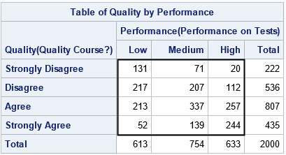
The previous article showed that you can specify the PLCORR option on the TABLES statement to estimate the polychoric correlation between Y1 and Y2. The estimate is r = 0.4273. In this article, we are going to obtain the same estimate by manually finding the value of the correlation that maximize the log-likelihood function.
Estimate threshold values for each variable
The previous article shows a graph that illustrates the geometry in which two latent bivariate normal variables are binned to obtain the observed ordinal variables. You must estimate the threshold values (or cutoff values) that convert the latent variables to the ordinal variables. The simplest way to obtain the threshold parameters is to use the normal QUANTILE function.
Suppose the observed cumulative proportions for Y1 are {u1, u2, ..., uk1}. (Notice that uk1=1.) If X1 is the latent standard normal variable that produces Y1, then you can estimate the threshold parameters for X1 as {a1, a2, ..., ak1}, where Φ(ai) = u1 and where Φ is the cumulative distribution function for the standard normal distribution. This implies that the Y1 ordinal variable is generated from the X1 normal variable by using the bins (-∞, a1], (a2, a3), ... (ak1-1, ∞). The k1-1 values a1 < a2 < ... < ak1-1 are the cut points for X1.
Similarly, if the cumulative proportions for Y2 are {v1, ..., vk2}, and X2 is the latent standard normal variable that produces Y2, then the bins (-∞, b1], (b2, b3), ... (bk2-1, ∞) generate Y2, where Φ(bi) = v1. The k2-1 values b1 < ... < bk2-1} are the cut points for X2.
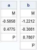
The following SAS IML statements read the marginal cumulative percentages, convert them to proportions, and compute the threshold values for each ordinal variable:
/* Download the PROBBVN function from https://github.com/sascommunities/the-do-loop-blog/blob/master/bivariate-normal-prob/ProbBnrm.sas See "Bivariate normal probability in SAS" https://blogs.sas.com/content/iml/2023/12/04/bivariate-normal-probability-sas.html */ proc iml; load module=(CDFBN ProbBVN); /* The cutoff points a[i] and b[i] are estimated from the empirical cumulative frequencies. */ use Y1Out; read all var {Y1 'cum_pct'}; close; u = cum_pct / 100; /* convert to proportion */ k1 = nrow(u); a = .M // quantile("Normal", u[1:k1-1]) // .P; use Y2Out; read all var {Y2 'cum_pct'}; close; v = cum_pct / 100; /* convert to proportion */ k2 = nrow(v); b = .M // quantile("Normal", v[1:k2-1]) // .P; print a[F=7.4], b[F=7.4]; |
Find the bivariate probability in each region
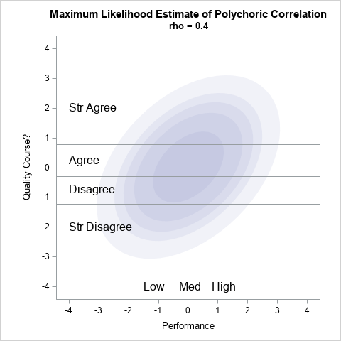
The thresholds define 12 rectangular regions in the plane, as shown in the graph to the right. For illustration, the graph shows the regions overlaid on a graph that is intended to represent the probability density of a bivariate normal distribution with correlation ρ = 0.4. In reality, we do not yet know what correlation best fits the data. As part of the estimation of the polychoric correlation, we must be able to calculate the total probability in each region for any value of ρ.
Mathematically, this calculation requires integrating the bivariate probability density over each region. Fortunately, SAS provides an easier way: You can use the built-in PROBBNRM function and some clever mathematical tricks to define an IML function that enables you to accurately calculate the total probability in each region. You can download this function (ProbBVN) from GitHub and use it as part of the estimation of the polychoric correlation.
Let's choose ρ=0.4 to illustrate the probability computation. For ρ=0.4, the following IML statements evaluate the bivariate normal probability for the rectangular regions that are defined by the threshold values for X1 and X2. This requires 12 calls to the ProbBVN function, which is performed in a loop:
/* show how to evaluate the probability that a BVN(0,rho) variate is in each region. For example, choose rho=0.4 */ rho = 0.4; pi = j(nrow(b)-1, nrow(a)-1, .); /* allocate matrix for results */ do i = 1 to nrow(b)-1; do j = 1 to nrow(a)-1; pi[i,j] = ProbBVN(a[j], a[j+1], b[i], b[i+1], rho); end; end; print pi[r=a c=b F=4.2]; |
In the resulting table of probabilities (not shown), the Y2 value increases as you move down the rows. But in the graph, the Y2 value points up. To make table similar to the graph, I reverse the rows of the matrix and printing the probabilities again:
/* reverse the rows so Y1 points up */ P = pi[nrow(pi):1, ]; print P[r={0.7807 -0.3081 -1.2212 .M} c={.M -0.5058 0.4775} F=4.2 L="Bivariate Normal Probability"]; |
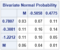
The values in the cells sum to 1 (in exact arithmetic) because together they account for all of the probability. The upper left corner of the table tells you that the probability is 0.03 that a random variate from the BVN(0, 0.4) distribution is observed in the upper-left quadrant of the graph, which corresponds to the "(Low, Strongly Agree)" ordinal group. The other 12 cells have similar meaning. For example, the upper right corner of the table tells you that the probability is 0.11 for the "(High, Strongly Agree)" ordinal group, which is the upper-right quadrant in the graph.
It is convenient to encapsulate the calculation of the probability matrix into a function:
/* compute the standard BVN probability for the rectangular regions defined by the vectors a and b. */ start ProbBVNMatrix(rho, _a, _b); a = colvec(_a); b = colvec(_b); pi = j(nrow(b)-1, nrow(a)-1, .); do i = 1 to nrow(b)-1; do j = 1 to nrow(a)-1; pi[i,j] = ProbBVN(a[j], a[j+1], b[i], b[i+1], rho); end; end; return pi; finish; /* test calling the ProbBVNMatrix function */ pi2 = ProbBVNMatrix(rho, a, b); |
The log-likelihood function
The log-likelihood function for polychoric correlation is easy to write down if you can compute the bivariate probabilities. The log-likelihood function (up to a constant) is the sum
\(
LL = \sum_{ij} n_{ij} \pi_{ij}
\)
where \(\pi_{ij}\) is the (i,j)th cell in the matrix of probabilities (when the rows are in the original order) and
where \(n_{ij}\) is the observed frequency of counts for the j_th level of Y1 and the i_th level of Y2.
The log-likelihood function can therefore be evaluated as the sum of the elementwise multiplication of the observed frequencies and the probabilities, given a value of ρ:
/* Find LL for the value of rho */ /* read the observed frequencies from the PROC FREQ output */ use FreqOut; read all var {'Count'}; close; n = shape(Count, nrow(Y2), nrow(Y1)); *print n[r=Y2 c=Y1]; /* evaluate LL for this value of rho */ LL = sum( n#log(pi) ); print rho LL; |
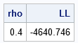
The computation shows that the log-likelihood when ρ=0.4 is -4641. So what does that mean? Not much by itself. The log-likelihood (LL) function is a function of the parameter ρ. For each ρ, it tells us how likely it is that the observed data come from the BVN(0, ρ) distribution, assuming the cut point values. So, the usefulness of the LL function lies in finding the ρ value that maximizes the LL. If you hold the cut points fixed, you can evaluate the LL for various values of ρ and visualize the shape of the LL function:
/* plot LL vs rho */ pi = j(nrow(n), ncol(n), .); rhos = T( do(0, 0.6, 0.01) ); /* choose some values of rho */ LL = j(nrow(rhos), 1); do k = 1 to nrow(rhos); pi = ProbBVNMatrix(rhos[k], a, b); /* probs for each rho value */ LL[k] = sum( n#log(pi) ); /* evaluate LL(rho) */ end; title "Loglikelihood for polychoric correlation"; call series(rhos, LL) grid={x y}; |
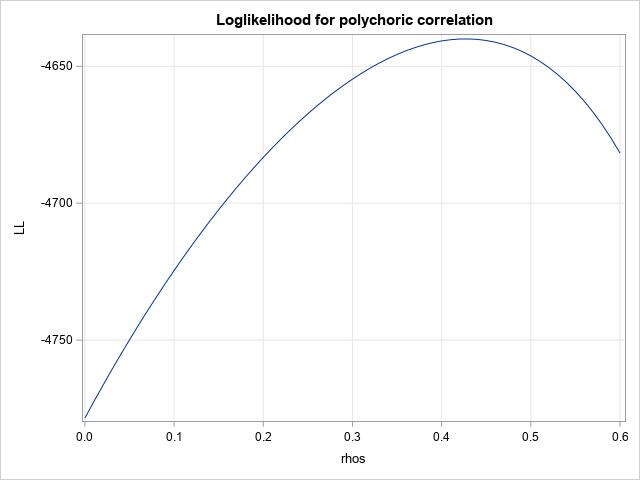
For this example, it looks like the maximum value of the log-likelihood function occurs when ρ ≈ 0.43. Therefore, the estimate of the polychoric correlation is about 0.43, assuming that the cut points are as specified.
One-parameter MLE for the polychoric correlation
Instead of graphing the LL function, you can use a one-parameter optimization to find the value of ρ that maximizes the LL. In SAS Viya, you can use the LPSOLVE subroutine to perform nonlinear optimization. In SAS 9.4, you can use the NLPNRA function to optimize the LL function. The LL function must use the observed frequencies and cutoff values, so these are defined as global variables. Although I don't do it here, you might want to constrain the correlation parameter to the interval [-0.99, 0.99] to avoid potential singularities for degenerate data.
/* MLE optimization of the LL objective function. See https://blogs.sas.com/content/iml/2011/10/12/maximum-likelihood-estimation-in-sasiml.html */ start LLPolychorRHO(rho) global( g_a, g_b, g_Freqs ); a = g_a; b = g_b; pi = ProbBVNMatrix(rho, a, b); LL = sum( g_Freqs#log(pi) ); return LL; finish; /* define global variables used in the optimization */ g_a = a; g_b = b; g_Freqs = n; /* set-up for Newton-Raphson optimization NLPNRA */ rho0 = 0.1; /* initial guess for solution */ opt = {1}; /* find maximum of function */ /* find optimal value of rho, given the data and cut points */ call nlpnra(rc, polycorrEst1, "LLPolychorRHO", rho0) opt=opt; print polycorrEst1; |

As shown by the graph of the LL function, the value of ρ that maximizes the LL is ρ = 0.4270.
Multi-parameter MLE for the polychoric correlation
Olsson (1974, p. 448) reports that early researchers used the polychoric correlation estimate in the previous section because "this approach has the advantage of reducing the computational labor" even though the estimate is "theoretically non-optimal." However, modern software provides a slightly more accurate estimate. Instead of assuming that the threshold value are fixed values, you can allow them to vary slightly. This results in a better estimate.
To get the better estimate, use the empirical threshold values and the correlation estimate in the previous section as the initial guess for a LL function that includes the parameters rho, a, and b. This requires optimizing k1+k2-1 parameters. The log-likelihood function is the same, but now the threshold values are considered as parameters, so they are passed into the objective function and removed from the GLOBAL clause. The new objective function is as follows:
/* the full objective function for LL of polychoric correlation */ start LLPolychor(param) global( g_Freqs ); /* param = rho // a // b */ k1 = ncol(g_Freqs)-1; /* num threshold params for X1 */ k2 = nrow(g_Freqs)-1; /* num threshold params for X2 */ rho = param[1]; a = .M // param[2:k1+1] // .P; b = .M // param[k1+2:1+k1+k2] // .P; pi = ProbBVNMatrix(rho, a, b); if any(pi<0) then return( . ); LL = sum( g_Freqs#log(pi) ); return LL; finish; |
By using this LL function, you can obtain the estimate for the polychoric correlation between two ordinal variables. First, optimize the LLPolychorRHO function by using the empirical values of the threshold parameters. Then, create a vector of parameters that contains the correlation (ρ) and the thresholds (a and b). Last, optimize the LLPolychor as a function of the parameters. You need to set up linear constraints so the solution respects the X1 threshold relationship a1 < a2 < ... < ak1-1, and similarly for the X2 thresholds:
/* Maximize the full log-likelihood function */ /* First, create initial guess from empirical thresholds and best rho value */ call nlpnra(rc, polycorr0, "LLPolychorRHO", rho0) opt=opt blc=con; param0 = polycorr0 // a[2:nrow(a)-1] // b[2:nrow(b)-1]; /* define global variables used in the optimization */ g_Freqs = n; /* set-up for Newton-Raphson optimization NLPNRA */ /* Second, set up contraint matrix -0.99 < rho < 0.99 0 < a[1] < a[2] < 1 0 < b[1] < b[2] < b[3] < 1 */ /* rho a1 a2 b1 b2 b3 op RHS*/ con = {-0.99 . . . . . . ., /* lower bounds */ 0.99 . . . . . . ., /* upper bounds */ 0 1 -1 0 0 0 -1 0, /* a1 < a2 */ 0 0 0 1 -1 0 -1 0, /* b1 < b2 */ 0 0 0 0 1 -1 -1 0}; /* b2 < b3 */ opt = {1, /* find maximum of function */ 1}; /* print some intermediate optimization steps */ /* Third, optimize the LL to estimate polychoric correlation */ call nlpnra(rc, polycorrEst2, "LLPolychor", param0) opt=opt blc=con; print polycorrEst2[c={'rho' 'a1' 'a2' 'b1' 'b2' 'b3'}]; |
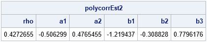
The output shows that the estimate of the polychoric correlation is 0.4273, which is the same value that is produced by PROC FREQ (and PROC CORR). Notice, however, that the manual computation gives additional information that is not provided by PROC FREQ. Namely, you get estimates of the threshold parameters! For this example, which has a sample size of 2,000 observations, the threshold parameters are not very different from the empirical values. The Newton-Raphson optimization only requires a few steps to converge from the initial guess because the initial guess is very close to the final optimal estimate. For smaller samples, the final estimate might be farther from the initial estimate.
Summary
Although the PLCORR option in PROC FREQ enables you to estimate the polychoric correlation of two ordinal variables, there is value in implementing the MLE optimization manually. This article shows how to implement the MLE algorithm in SAS IML to obtain the polychoric correlation estimate. Programming an algorithm yourself leads to a better understanding of the statistic and its assumptions. It also enables you to build skills that can be used to compute statistics that SAS does not provide. This example also shows the power and flexibility of the SAS IML language to implement methods in computational statistics.
You can download the SAS program that creates all tables and graphs in this article from GitHub.
