A previous article shows how to use Monte Carlo simulation to approximate the sampling distribution of the sample mean and sample median. When x ~ N(0,1) are normal data, the sample mean is also normal, and there are simple formulas for the expected value and the standard error of the mean. These formulas are provided in elementary statistics courses.

It turns out that when the data are normal, the distribution of the sample median is also known explicitly, although the formulas are not simple. Fortunately, SAS provides the PROBMED function, which enables you to evaluate the CDF of the distribution of the sample median. From the CDF, you can obtain the PDF, the quantile function, and random variates. This article shows how to use the PROBMED function in SAS to visualize the distribution of the sample median of normally distributed data.

The distribution of the sample median

For random samples of size n drawn from a normal distribution, there is an exact formula for the cumulative distribution function (CDF) of the sample median. The formula is given in the documentation of the PROBMED function.

When n is an odd integer, the CDF is defined in terms of the incomplete beta function. The following DATA step calls the PROBMED function to compute the CDF for the sampling distribution of the median in normal samples of various sizes (all odd integers). The PDF is approximated by using a forward finite-difference approximation to the derivative of the CDF.

/* PROBMED is the CDF of the sampling distribution of the
sample median for normally distributed N(0,1) data of size n */
data MedianCDF;
dx = 0.01;
do n = 11, 21, 31, 51;
   firstObs = 1;
   do x = -1.5 to 1.5 by dx;
      CDF = probmed(n, x);
      PDF = dif(CDF) / dx;     /* finite-diff approx to PDF */
      if firstObs then do;
         PDF = .;
         firstObs = 0;
      end;
      output;
   end;
end;
run;
 
title "CDF of the Sampling Distribution of the Sample Median";
title2 "Size n; x ~ N(0,1)";
proc sgplot data=MedianCDF;
   series x=x y=CDF / group=n;
   xaxis grid;
   yaxis grid;
run;

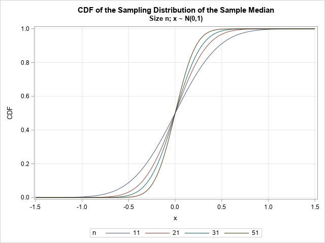
The graph shows the CDF for increasingly larger values of the sample size, n. For larger samples, the distribution is more concentrated near x=0, which is the median of the underlying N(0,1) distribution for x. This is better visualized if you plot the PDF curves, as follows:

title "PDF of the Sampling Distribution of the Sample Median";
title2 "Size n; x ~ N(0,1)";
proc sgplot data=MedianCDF;
   series x=x y=PDF / group=n;
   xaxis grid;
   yaxis grid;
run;

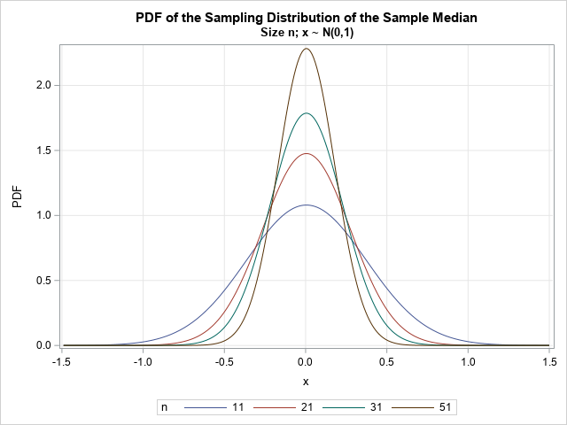
The graphs of the PDFs show that the sample median has more variation in small samples and less variation in larger samples.

The distribution for even-sized samples

I used odd values for n because the formula is simpler to understand, but the PROBMED function supports even values of n as well. Feel free to regenerate the images for even values of n.

The exact PDF for odd-sized samples

To compute the PDF, I used a forward finite-difference approximation to the derivative of the CDF. This works for samples of any size. However, when n is odd, it's possible to compute an exact formula for the PDF by taking the derivative with respect to x of the formula for the CDF. You can obtain the derivative by applying the Fundamental Theorem of Calculus and the chain rule to the formula for the CDF. The following DATA step is an exact computation of the PDF when n is an odd integer:

/* write explicit formula for PDF when sample size is any ODD integer */
data MedianPDF;
n = 11;
a = (n+1)/2;
do x = -1.5 to 1.5 by 0.01;
   PhiX = cdf("Normal", x);                /* Phi(x) is upper limit of integral */
   CDFBeta = cdf("Beta", PhiX, a, a);      /* the scaled incomplete beta fcn at Phi(x) */
   /* use FTC + chain rule to obtain the PDF */
   PDF = pdf("Beta", PhiX, a, a) * pdf("Normal",x);   
   output;
end;
run;

If you need to use the exact formula, you can put that formula into a user-defined function or into a macro, as follows:

%macro PDFMedOdd(x, n);
    pdf("Beta", cdf("Normal", &x), (&n+1)/2, (&n+1)/2) * pdf("Normal",&x)
%mend;

The PDF formula for sample sizes that are even integers is more complicated. You can't apply the fundamental theorem of calculus because the integrand is a function of x. Thus, for even n, you must evaluate the integral numerically for each value of x.

Quantiles of the sampling distribution

You can invert the CDF function to find the quantile function. For any sample size, n, and for a given probability, p, you can find the quantile by solving for a root: Find x such that PROBMED(n, x) - p = 0. The details (and a SAS IML program) are given in a previous article about finding quantiles.

For sample sizes that are odd integers, you can explicitly invert the CDF function and obtain the quantile function as the composition of the quantile functions of a beta and a normal distribution. The following SAS statements evaluate the explicit quantile:

/* use built-in QUANTILE function to find the exact quantile when the sample size is ODD */
a = (&n+1)/2;
qBeta = quantile("Beta", probs, a, a);
q = quantile("Normal", qBeta);

Random variates

Whether you use a root-finding algorithm or an explicit formula to obtain the quantile function, you can obtain random variates from the quantile function. In either case, you can use the inverse CDF method to generate random variates from the sampling distribution.

Summary

Base SAS supports the PROBMED function, which evaluates the CDF of the sampling distribution for the median of a normally distributed data set of size n. You can use the function to evaluate probabilities (p values) and to construct confidence intervals for the sample median.

SAS does not explicitly provide the PDF or quantile function for this distribution. However, this article shows that you can use finite-difference approximation to obtain the PDF function, or you can explicitly differentiate the CDF formula. I show the derivative for even samples, which is the easy case. Similarly, you can use a root-finding algorithm to obtain the quantile function, or you can explicitly invert the CDF formula. From the quantile function, you can generate random variates.