An elementary course in statistics often includes a discussion of the sampling distribution of a statistic. The canonical example is the sampling distribution of the sample mean. For samples of size n that are drawn from a normally distribution (X ~ N(μ, σ)), the sample mean is normally distributed as m ~ N(μ, σ/sqrt(n)), where m is the sample mean. (Note: For normal data, the sampling distribution of the mean is also normal. You do not need to invoke the Central Limit Theorem.)

Elementary courses do not discuss the sampling distribution of the sample median because that statistic has a much more complicated sampling distribution. However, you can use simulation to approximate the sampling distribution of the median and to estimate inferential quantities such as the standard error or a confidence interval.

This article shows how to use a simulation to approximate the sampling distribution of the median. A second article shows how to compute the exact distribution of the sample median for normally distributed data.

Standard error and confidence interval for the sample mean

Before we discuss the sample median, let's review the distribution of the sample mean. For a normally distributed sample of size n, the sampling distribution of the sample mean is well known. The formulas are given in elementary statistics courses. The following SAS DATA step evaluates the standard formulas for samples of size n:

%let n = 11;                   /* n = sample size */
 
data MeanFormula;              /* evaluate SEM and CI for x ~ N(0,1) and n=11 */
mu = 0; sigma = 1;             /* assume x ~ N(mu, sigma) */
EMean = mu;                    /* expected value of mean */
seMean = sigma / sqrt(&n);     /* standard error of the mean */
alpha = 0.1;                   /* compute 90% CI for the mean */
zCrit = quantile("normal", 1-alpha/2);    
LowerCL = mu - seMean * zCrit;
UpperCL = mu + seMean * zCrit;
run;
 
proc print data=MeanFormula noobs; 
   var EMean seMean LowerCL upperCL;
run;

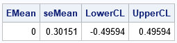
The output shows the results of evaluating the classic formulas when x ~ N(0,1) and n=11. The sample mean is normally distributed with expected value 0 and standard error 0.302. The formula for a symmetric 90% probability interval is also provided. (This interval estimate is usually given in terms of the sample statistics; I've used the population parameters.) The computation shows that most samples from N(0,1) will have a mean in the range [-0.496, 0.496]. The next section shows how to use simulation to obtain similar values.

Why use n=11? It is an odd number, therefore the median is the middle data value.

A SAS simulation of statistics for normal data

If you are not familiar with simulating data with SAS, see a previous article that shows how to use simulation to approximate the sampling distribution of the sample mean. By changing a few lines of the program, you can simultaneously approximate the sampling distribution of the median. The following program simulates 10,000 normally distributed samples of size n=11. For each sample, the sample mean and median are computed. The final table shows the summary statistics for the distribution of the sample mean and sample median:

/* Use simulation to find the distribution of the sample 
   mean and median for normally distributed N(0,1) samples. */
%let n = 11;             /* n = sample size */
%let NumSamples = 10000;  /* number of simulated samples */
/* 1. create many normally distributed samples of size n */
data SimNormal(keep=SampleID x); 
call streaminit(123);
do SampleID = 1 to &NumSamples;  
   do i = 1 to &n;               
      x = rand("Normal");
      output;
   end;
end;
run;
 
/* 2. compute mean and median for each N(0,1) sample */
proc means data=SimNormal noprint; 
   by SampleID;
   var x;
   output out=OutStats mean=SampleMean median=SampleMedian;
run;
 
/* 3. analyze the sampling distribution of the statistics */
proc means data=OutStats N Mean StdDev P5 P95;
   var SampleMean SampleMedian;
run;

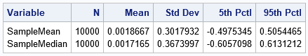
The output shows Monte Carlo estimates for the distributions of the sample mean and sample median in samples of size n=11 when x ~ N(0,1). This output does not use any information about the true parameters. For the sample mean, the first row shows that the expected value is close to 0, and the standard error is 0.302. A 90% confidence interval (CI) is [-0.498, 0.505]. These values are close to the results of the formulas in the previous section.

The corresponding Monte Carlo estimates for the sample median are shown in the second row. Again, the expected value is 0, but the standard error for the median is larger (0.367) than for the mean. Similarly, the 90% CI is wider: [-0.601, 0.613].

Compare the sampling distribution of the mean and median

The previous table shows summary statistics for the sampling distributions of the mean and median. However, you can also use the simulation to visualize the Monte Carlo approximations to the sampling distributions. The following call to PROC SGPLOT displays a density estimates for the sampling distribution of each statistic. In accordance with theory, a normal density is used to visualize the distribution of the sample mean. A kernel density estimate is used to visualize the distribution of the median:

title "Sampling Distribution of the Sample Mean and Median";
title2 "n = &n; x ~ N(0,1)";
proc sgplot data=OutStats;
   density SampleMean / type=Normal legendlabel="Mean";
   density SampleMedian / type=Kernel legendlabel="Median";
   xaxis grid;
   yaxis grid;
run;

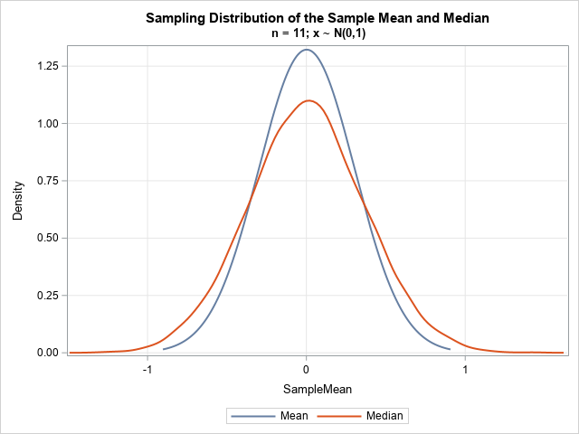
The graph overlays the distributions for the sample mean and sample median. The distribution of the median is wider. The distribution of the median looks to be approximately normal, but it is hard to draw conclusions from a single simulation study. In the next article, I will construct an exact distribution for the sample median of normal data.

The sampling distributions for non-normal data

One great thing about simulation studies is that you can approximate sampling distributions of statistics when the theoretical distribution is unknown or very complicated to compute. As an example, suppose we want to approximate the sampling distributions for exponential data. That is, if x ~ Expon(1), what is the sampling distribution of the mean and median in samples of size 11?

You only need to change one line in the previous simulation. In the DATA step that simulates the data, use x = rand("Expo") to simulate exponential variates (n=11). Because exponential data is not as tame as normal data, I also suggest increasing the number of Monte Carlo samples by using NumSamples = 100000. With those two modifications, the following table and graph approximate the distribution of the sample mean and median in exponential data:

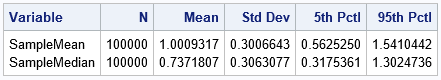
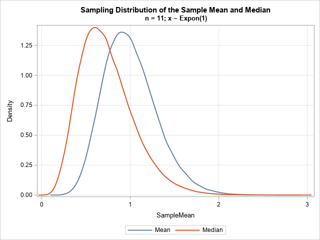
The exponential distribution has a long right tail, so we expect the same for the sampling distributions. For the (standard) exponential distribution, the mean is 1, and the median is log(2) ≈ 0.693. Therefore, we expect the modes of the sampling distributions to be different from each other. An analysis of the sampling distributions is beyond the scope of this article. I merely want to demonstrate that you can use simulation to approximate the distribution of statistics for non-normal data.

Summary

This article shows how to compare the distribution of the sample mean and sample median for normal and non-normal data. The article uses a small sample (n=11), but the simulation can handle larger samples. For normal data, the distribution of the median is wider than the distribution of the mean, but they have similar shapes. For non-normal data, the two distributions can look quite different.

It turns out that there is an exact (but complicated) formula for the exact distribution of the sample median for normally distributed data. That formula is discussed in a second article.