A previous article shows an example of a Markov chain model and computes the probability that the system ends up in a terminal state (called an absorbing state). As explained previously, you can often compute exact probabilities for questions about Markov chains. Nevertheless, it can be useful to know how to simulate from a Markov system and to use the simulation to compute Monte Carlo estimates for probabilities. This article shows how to use SAS IML to simulate samples from a Markov model.

A simple Markov model

Let's reuse the example from my previous article. The system is defined by a 4 x 4 transition matrix. The first row contains the transition probabilities for State 1, the second row contains the probabilities for State 2, and so on. See the previous article for a description of the system in terms of a game that involves flipping a fair coin.

proc iml;
/* Transition matrix. Columns are next state; rows are current state */
/*     Null  H   HT  HTH */
P =    {0.5  0.5 0   0,   /* Null */
        0    0.5 0.5 0,   /* H    */
        0.5  0   0   0.5, /* HT   */
        0    0   0   1};  /* HTH  */

Simulate from a Markov model

In this example, the initial state is always State=1. The first row of the transition matrix specifies that the next state will be 1 or 2 with equal probability. You can use the "Table" distribution in the RANDFUN function to simulate the next state from a vector of probabilities. Let k be the state returned by the RANDFUN function. Then you can simulate the next state by using the probabilities in the kth row of the transition matrix in a call to the RANDFUN("TABLE") function. You can repeat this process to obtain a sequence of states, as shown in the following SAS IML statements:

/* simulate the first 10 states for the game */
call randseed(1235);
maxN = 10;
state = j(maxN, 1, .);
state[1] = 1;       /* every new game begins in State 1 */
do i = 2 to maxN;
   probTrans = P[state[i-1], ];               /* vector of transition probs for current state */
   state[i] = randfun(1, "Table", probTrans); /* simulate next state */
end;
print state[r=(0:maxN-1)];

One possible realization of the process is shown. Initially, the system is in State=1. For this seed value, the state of the system evolves according to the sequence 2, 2, 3, 1,.... Eventually, the system reaches State=4, which is the terminal state. Subsequent iterations of the system will always be in State=4, as seen by looking at the last row of the transition matrix.

Because the system will stay in State=4, you can replace the DO loop with a DO-UNTIL loop that breaks out of the loop if the system reaches State=4. This is shown in the following function definition, which simulates data from a Markov chain starting from an initial state:

/* Simulate a Markov process. If there is a terminal event 
  (eg, death), jump out of the loop if reached. 
  INPUT:
  maxN:      maximum number of states of the system
  initState: inital state for system
  P:         a (k x k) transition matrix. The i_th row is the 
             probability vector for transitioning from the i_th state.
  termState: (optional) stop the simulation if State becomes termState
  OUTPUT:  The function returns an Nx1 vector of states. If the system reaches a terminal 
           state, the last entries are missing values.
*/
start SimMarkov(maxN, initState, P, termState=.);
   state = j(maxN, 1, .);
   state[1] = initState;
   do i = 2 to maxN until(state[i]=termState);
      probTrans = P[state[i-1], ];     /* transition prob for current state */
      state[i] = randfun(1, "Table", probTrans);
   end;
   return state;
finish;
 
/* test the function by simulating states */
maxN = 10;
state = SimMarkov(maxN, 1, P, 4); /* init state=1; terminal state=4 */
print state[r=(0:maxN-1)];

The call to the SimMarkov function simulates the system and puts the results in the state vector. In this simulation, the ninth state of the system is State=4. Because State=4 is the terminal state, the 10th element of the return vector is a missing value.

Simulating many trials from a Markov process

To simulate B independent realizations of the stochastic process, call the SimMarkov function multiple times and fill B columns of a matrix. For example, the following call simulates B=5 random draws from the same Markov process. For brevity, I have simulated only the first 10 states:

/* simulate B trials, each with up to N states */
N = 10;       /* maximum number of transitions */
B = 5;        /* number of random draws */
state = j(N, B, .);
do j = 1 to B;
   state[ ,j] = SimMarkov(N, 1, P, 4); /* init state=1; terminal state=4 */
end;
print state[r=(0:N-1) c=('Trial1':'Trial5')];

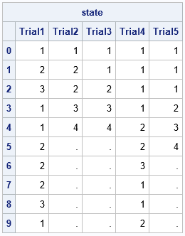
In these simulations, the second, third, and fifth trials terminated before the 10th state. The first and fourth trials did not reach the terminal state within 10 states (or 9 transitions).

Use simulation to estimate probabilities

As mentioned earlier, you can often compute exact probabilities for Markov chains. Notice the difference between the number of states and the number of transitions. In the previous tables, I have labeled the initial state with '0' to indicate that the system has not experienced any transitions. The second row indicates the state after the first transition. In general, the i_th row shows the state after i-1 transitions. Because the system always starts in State=1, it is easier to use the number of transitions (not states) to compute probabilities.

A previous article computes the distribution for the random variable N, which is defined as the number of transitions before the system reaches the terminal state. Let's run a large simulation study and use the simulated trials to estimate the probabilities that were computed in the previous article. First, run the simulation:

/* Simulate 10,000 indep trials. Use simulation to estimate probabilities. */
B = 10000;
maxN = 40;
state = j(maxN+1, B, .);
do j = 1 to B;
   state[ ,j] = SimMarkov(maxN+1, 1, P, 4); /* init state=1; terminal state=4 */
end;
state = state[2:maxN+1, ];    /* delete the initial state, which is always 1 */

Now use the 10,000 simulated trials to estimate the distribution of N. You can estimate the density of the distribution of N by using the proportion of columns for which State=4 appears on row 1, 2, 3, 4, ..., as follows:

/* 1. estimate the probability distribution */
termState = 4;
numTransitions = T(1:maxN);
Freq = j(maxN, 1, 0);
do i = 1 to maxN;
   Freq[i] = sum(state[i, ]=termState);
end;
EstDensity4 = Freq / B;
 
/* visualize the distribution by graphing the probability density */
create EstMarkov var {'numTransitions' 'EstDensity4'}; append; close;
submit;
title "Estimated Density for Terminal State";
proc sgplot data=EstMarkov;
   needle x=numTransitions y=EstDensity4 / lineattrs=(thickness=7);
   yaxis grid label='Estimated Density';
   xaxis label='Number of Transitions';
run;
endsubmit;

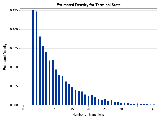
The graph visualizes the estimated probability mass function for the random variable N. The simulation-based estimate of the distribution is close to the exact distribution, which was computed in the previous article. However, you can see that the estimated distribution is more jagged than the exact distribution. In the exact distribution, the probabilities in the tail are strictly decreasing. Nevertheless, this estimate shows the approximate shape of the distribution.

After you have estimated the probability distribution, other computations are straightforward. The next computation estimates the expected value of N by using the empirical probabilities from the simulation. A subsequent computation estimates the number of transitions required until the system has a 99% chance of reaching the terminal state.

/* 2. The expected length of a trial (approx by using maxN=40 turns) */
EstELen = EstDensity4`*numTransitions;
print EstELen[L='Est E[Length]' F=5.3];
 
/* 3. Find n such that Pr(N <= n) >= 0.99 */
estProb = cusum(EstDensity4);      /* estimate of cumulative probability */
est99 = loc(estProb >= 0.99)[1];
print est99;

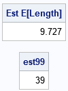
For these 10,000 simulated samples, there is an average of 9.727 transitions until the system reaches the final state. The computation gives 39 as an estimate for the number of transitions before there is a 99% chance of being in State=4. For comparison, if you use the exact probability, the estimates are 9.673 and 38, respectively. If you run more simulations, the Monte Carlo estimates become closer to the exact probabilities.

Summary

You can often compute exact probabilities for questions about Markov chains. However, it can be useful to know how to simulate from a Markov system. This article shows how to use SAS IML to simulate many samples from a Markov model. You can use the simulation to compute Monte Carlo estimates for some probabilities. The Monte Carlo estimates are close to the true probability values.