A previous article shows how to model the probabilities in a discrete-time Markov chain by using a Markov transition matrix. A Markov chain is a discrete-time stochastic process for which the current state of the system determines the probability of the next state. In this process, the probabilities for transitioning to the next state depend only on the current state.

As shown previously, if you specify the initial state of the system, you can use matrix-vector multiplication to obtain the probability that the system will be in each state after t transitions, t = 1, 2, ..., N. For some systems, there is a final or terminal state. When the system enters that state, it remains in that state for all time. Such a state is called an absorbing state. A canonical example of a terminal state occurs in epidemiological models for the transmission of a disease. A subject might be in one of four states: Susceptible, Infected, Recovered, and Dead. The Dead state is absorbing because there are no transitions out of that state.

I previously wrote about absorbing states by analyzing the system with the tools of linear algebra. However, it is also useful to use probability theory to understand absorbing states. This article uses an example that has four states to illustrate how you can compute exact probabilities that enable you to answer questions about how long it takes the system to enter the absorbing state. This article uses the SAS IML language to perform the computations, but the results are similar in other languages that support matrix-vector computations.

A simple Markov model

Let's reuse the example from my previous article, which is also used by the A Wikipedia article on Markov chains. The Markov chain models a game in which you toss a fair coin until the sequence heads-tails-heads (HTH) appears. The process has the following four states:

• State 1: No elements of the sequence are in order. If the next toss is tails (T), the system stays at State 1. If the next toss is heads (H), the system transition to State 2.
• State 2: H. The first element of the sequence is in order. If the next toss is H, the system stays at State 2. If the next toss is T, the system transitions to State 3.
• State 3: HT. The first two elements of the sequence in order. If the next toss is H, transition to State 4. If the next toss is T, transition to State 1.
• State 4: HTH. The game is over. Stay in this state.

The transition matrix is given by the following SAS IML matrix. The first row contains the transition probabilities for State 1, the second row contains the probabilities for State 2, and so on.

proc iml;
/* Transition matrix. Columns are next state; rows are current state */
/*     Null  H   HT  HTH */
P =    {0.5  0.5 0   0,   /* Null */
        0    0.5 0.5 0,   /* H    */
        0.5  0   0   0.5, /* HT   */
        0    0   0   1};  /* HTH  */

Almost surely, all systems eventually end up in State=4, which is the absorbing state. An interesting question is how many transitions (on average) does the system make before it reaches State=4? In general, what is the probability that the system reaches the terminal state after 3, 4, 5, ... transitions from the initial state?

Let's ask and answer three questions about the number of transitions, N, that the system will go through before reaching its terminal state. The quantity N is a random variable, so it has a distribution.

1. What is the distribution of N? That is, what is the probability that the system will reach its terminal state after 3, 4, 5, ... transitions?
2. What is the expected value of N? That is, on average, how many transitions does it take until the system reaches its terminal state?
3. For what value of N does the system reach its terminal state at least 99% of the time? That is, find n such that Pr(N ≤ n) ≥ 0.99.

These question all rely on being able to compute the distribution of N. Although is is theoretically possible that the system might never reach the terminal state, in practice, the system is very likely to reach its terminal state after sufficiently many transitions. The definition of "sufficiently many" will be decided by answering the third question. For now, let's use a maximum of 40 transitions to answer these questions.

QUESTION 1: The following computation iterates the transition matrix to compute the exact probability that the system is in each state after 1, 2, 3, ..., 40 transitions. A previous article includes a visualization of these probabilities. Notice that the following computations does NOT include the initial state, so the i_th row of the resulting matrix represents the probability after i transitions.

/* COMPUTATIONS THAT USE EXACT PROBABILITIES */
/* 1. What is the distribution N? */
maxN = 40;
Prob = j(4, maxN, .);  /* probability for each state */
v = {1,0,0,0};         /* start in State 1 */
do i = 1 to maxN;
   v = P`*v;           /* prob of state after i transitions */
   Prob[,i] = v;
end;
 
CumProb4 = Prob[4,];       /* cumulative distribution of N */
Density4 = dif(CumProb4);  /* PDF = change in CDF */
Density4[1] = 0;           /* replace missing value with  0 */
numTransitions = T(1:maxN);
 
/* write density to SAS data set and use needle plot to visualize
   https://blogs.sas.com/content/iml/2014/06/23/creating-ods-graphics-from-the-sasiml-language.html */
create Markov var {'numTransitions' 'Density4' 'CumProb4'}; append; close;

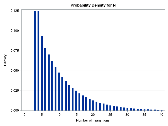
The graph visualizes the probability mass function for the random variable N. You can see that the most probable ending state is three or four transitions. As more and more transitions occur, the probability of reaching the terminal state for the first time decreases. See the Appendix for the SAS statements that create the graph.

QUESTION 2: What is the expected value of N? The expected value is the weighted mean of the number of transitions, with the weights given by the probability that the random variable takes each value. As a formula, $\text{E}[N] = \sum_i n_i f(n_i)$, where f is the discrete probability density function. This is an infinite sum, but we can approximate it by using a partial sum that uses a large number of terms. For this example, I will use a total of 40 terms:

/* 2. What is the expected value of N? */
ELen = Density4`*numTransitions;
print ELen[L='E[Length] (Approx)' F=5.3];

The approximate answer is that we should expect an average of 9.673 transitions before the game ends. This computation underestimates the true value, since the game can require more than 40 transitions, but as the graph shows, the probability of those cases is very small.

QUESTION 3: Find a value of n such that Pr(N ≤ n) ≥ 0.99. This question can be answered by looking at the cumulative distribution for N, which was previously computed as the fourth row of the Prob matrix. The following statement finds the first column for which the probability exceeds 0.99.

/* 3. Find n such that Pr(N <= n) >= 0.99.  */
N99 = loc(Prob[4,] > 0.99)[1];
print N99;

There is a 99% chance that the game ends on or before the 38th transition. This is why 40 transitions are used in the computations.

Summary

You can use matrix multiplication to compute the probability that a Markov process (represented by its transition matrix) is in each state after N transitions when the system starts in a given state. This article looks at a stochastic system that has four states and always starts in the first state. The fourth state is absorbing, which means that it is a terminal state. This article shows how to compute the exact probabilities for the distribution of N, the number of transitions before the system reaches the terminal state. After you compute the distribution of N, you can use it to answer related questions such as the expected value of N or the number of transitions that are required before the system has a 99% chance of reaching the terminal state.

Appendix: Visualizing the distribution of N

For completeness, here are the SAS statements that visualize the cumulative distribution and the density function of N, the number of transitions before the state reaches the terminal state (State=4).

title "Cumulative Probability for N";
proc sgplot data=Markov;
   needle x=numTransitions y=CumProb4 / lineattrs=(thickness=7);
   yaxis grid label='Probability';
   xaxis grid label='Number of Transitions' values=(0 to 40 by 5);
run;
 
title "Probability Density for N";
proc sgplot data=Markov;
   needle x=numTransitions y=Density4 / lineattrs=(thickness=7);
   yaxis grid label='Density';
   xaxis label='Number of Transitions' values=(0 to 40 by 5);
run;