Last week I showed how to represent a Markov transition matrix in the SAS/IML matrix language. I also showed how to use matrix multiplication to iterate a state vector, thereby producing a discrete-time forecast of the state of the Markov chain system. This article shows that the expected behavior of a Markov chain can often be determined just by performing linear algebraic operations on the transition matrix.

Absorbing Markov chains

Whereas the system in my previous article had four states, this article uses an example that has five states. The ith row of the following transition matrix gives the probabilities of transitioning from State i to any other state:

proc iml;
/* i_th row contains transition probabilities from State i */
P = { 0    0.5  0    0.5  0,
      0.5  0    0.5  0    0,
      0    0.5  0    0    0.5,
      0    0    0    1    0,
      0    0    0    0    1 };

For example, the last row of the matrix indicates that if the system is in State 5, the probability is 1 that it stays in State 5. This is the definition of an absorbing state. An absorbing state is common for many Markov chains in the life sciences. For example, if you are modeling how a population of cancer patients might respond to a treatment, possible states include remission, progression, or death. Death is an absorbing state because dead patients have probability 1 that they remain dead. The non-absorbing states are called transient. The current example has three transient states (1, 2, and 3) and two absorbing states (4 and 5).

If a Markov chain has an absorbing state and every initial state has a nonzero probability of transitioning to an absorbing state, then the chain is called an absorbing Markov chain. The Markov chain determined by the P matrix is absorbing. For an absorbing Markov chain, you can discover many statistical properties of the system just by using linear algebra. The formulas and examples used in this article are taken from the online textbook by Grimstead and Snell.

The first step for analyzing an absorbing chain is to permute the rows and columns of the transition matrix so that all of the transient states are listed first and the absorbing states are listed last. (The P matrix is already in this form.) If there are k absorbing states, the transition matrix in block form looks like the following:

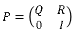
The bottom right block of the transition matrix is a k x k identity matrix and represents the k absorbing states. The top left block contains the probabilities of transitioning between transient states. The upper right block contains the probabilities of transitioning from a transient state to an absorbing state. The lower left block contains zeros because there is no chance of transitioning from an absorbing state to any other state.

The following SAS/IML statements show how to extract the Q and R matrices from the P matrix:

k = sum(vecdiag(P)=1);      /* number of absorbing states */
nt = ncol(P) - k;           /* number of transient states */
 
Q = P[1:nt, 1:nt];          /* prob of transitions between transient states */ 
R = P[1:nt, nt+1:ncol(P)];  /* prob of transitions to absorbing state */

Expected behavior of absorbing Markov chains

By definition, all initial states for an absorbing system will eventually end up in one of the absorbing states. The following questions are of interest. If the system starts in the transient state i, then:

1. What is the expected number of steps the system spends in transient state j?
2. What is the expected number of steps before entering an absorbing state?
3. What is the probability that the system will be absorbed into the jth absorbing state?

The answers to these questions are obtained by defining the so called fundamental matrix, which is N = (I-Q)^-1. The fundamental matrix answers the first question because the entries of N are expected number of steps that the system spends in transient state j if it starts in transient state i:

transState = char(1:nt);        /* labels of transient states */
absState = char(nt+1:ncol(P));  /* labels of absorbing states */
 
/* Fundamental matrix gives the expected time that the system is 
   in transient state j if it starts in transient state i */
N = inv(I(nt) - Q);  
print N[L="Expected Time in State j" r=transState c=transState];

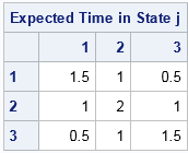
The first row indicates that if the system starts in State 1, then on average it will spend 1.5 units of time in State 1 (including the initial time period), 1 unit of time in State 2, and 0.5 units of time in State 3 before transitioning to an absorbing state. Similarly, if the system starts in State 2, you can expect 1 unit, 2 units, and 1 unit of time in States 1, 2, and 3, respectively, before transitioning to an absorbing state.

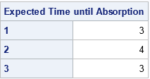
Obviously, if you sum up the values for each row, you get the expect number of steps until the system transitions to an absorbing state:

/* Expected time before entering an absorbing state if the system
   starts in the transient state i */
t = N[,+];
print t[L="Expected Time until Absorption" r=transState];

The remaining question is, to me, the most interesting. If the system starts in a transient state, you know that it will eventually transition into one of the k absorbing states. But which one? What is the probability that the system ends in the jth absorbing state if it starts in the ith transient state? The answer is obtained by the matrix multiplication N*R because the matrix N is the expected number of steps in each transient state and R contains the probability of transitioning from a transient state to an absorbing state. For our example, the computation is as follows:

/* The probability that an absorbing chain will be absorbed
   into j_th absorbing state if it starts in i_th transient state */
B = N*R;
print B[L="Absorption Probabilities" r=transState c=absState];

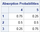
The first row of the matrix indicates that if the system starts in State 1, it will end up in State 4 three quarters of the time and in State 5 one quarter of the time. The second rows indicates that if the system starts in State 2, there is a 50-50 chance that it will end up in State 4 or State 5.

Because this Markov chain is a stochastic process, you cannot say with certainty whether the system will eventually be absorbed into State 4 or State 5. However, starting the system in State 1 means that there is a higher probability that the final state will be State 4. Similarly, starting in State 3 means a higher probability that the final state will be in State 5.

There are many other statistics that you can compute for absorbing Markov chains. Refer to the references for additional computations.

References

• The Wikipedia article "Absorbing Markov Chains"
• Grimstead and Snell, Chapter 11, "Markov Chains in Introduction to Probability