Many computations in elementary probability assume that the probability of an event is independent of previous trials. For example, if you toss a coin twice, the probability of observing "heads" on the second toss does not depend on the result of the first toss.

However, there are situations in which the current state of the system determines the probability of the next state. A stochastic process in which the probabilities depend on the current state is called a Markov chain.

A Markov transition matrix models the way that the system transitions between states. A transition matrix is a square matrix in which the (i,j)th element is the probability of transitioning from state i into state j. The sum of each row is 1. For reference, Markov chains and transition matrices are discussed in Chapter 11 of Grimstead and Snell's Introduction to Probability.

A transition matrix of probabilities

A Wikipedia article on Markov chains uses a sequence of coin flips to illustrate transitioning between states. This blog post uses the same example, which is described below.

Imagine a game in which you toss a fair coin until the sequence heads-tails-heads (HTH) appears. The process has the following four states:

• State 1: No elements of the sequence are in order. If the next toss is tails (T), the system stays at State 1. If the next toss is heads (H), the system transition to State 2.
• State 2: H. The first element of the sequence is in order. If the next toss is H, the system stays at State 2. If the next toss is T, the system transitions to State 3.
• State 3: HT. The first two elements of the sequence in order. If the next toss is H, transition to State 4. If the next toss is T, transition to State 1.
• State 4: HTH. The game is over. Stay in this state.

The transition matrix is given by the following SAS/IML matrix. The first row contains the transition probabilities for State 1, the second row contains the probabilities for State 2, and so on.

proc iml;
/* Transition matrix. Columns are next state; rows are current state */
/*     Null  H   HT  HTH */
P =    {0.5  0.5 0   0,   /* Null */
        0    0.5 0.5 0,   /* H    */
        0.5  0   0   0.5, /* HT   */
        0    0   0   1};  /* HTH  */
states = "1":"4";
print P[r=states c=states L="Transition Matrix"];

Analyzing sequences of coin tosses can be interesting and sometimes counterintuitive. Let's describe the expected behavior of this system.

The state vector

You can use a four-element row vector to represent the probabilities that the system is in each state. If the system is in the ith state, put a 1 in the ith element and zero elsewhere. Thus the state vector {1 0 0 0} indicates that the system is in State 1.

The time-evolution of the system can be studied by multiplying the state vector and the transition matrix. If s is the current state of the system, then s*P gives the vector of probabilities for the next state of the system. Similarly, (s*P)*P = s*P² describes the probabilities of the system being in each state after two tosses. (If you prefer to represent the state by using a column vector, v, then the probabilities are P`*v, (P<sup>2</sup>)`*v, and so forth.)

For the HTH-sequence game, suppose that you start a new game. The game starts in State 1. The following computation describes the evolution of the state vector:

s0 = {1 0 0 0};    /* a new game is in State 1 */
s1 = s0 * P;       /* probability distribution of states after 1 toss */
s2 = s1 * P;       /* probability distribution of states after 2 tosses */
print (s1//s2)[L="Prob of State" c=("1":"4") r={"1 toss" "2 tosses"}];

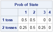
The first row of the output gives the state probabilities for the system after one coin toss. The system will be in State 1 with probability 0.5 (if you toss T) and will be in State 2 with probability 0.5 (if you toss H). The second row is more interesting. The computation use the probabilities from the first toss to compute probabilities for the second toss. After two tosses, the probability is 0.25 for being in State 1 (TT), the probability is 0.5 for being in State 2 (TH or HH), and the probability is 0.25 for being in State 3 (HT).

Modeling a sequence of coin tosses

In general you can repeatedly multiple the state vector by the transition matrix to find the state probabilities after k time periods. For efficiency you should avoid concatenating results inside a loop. Instead, allocate a matrix and use the ith row to hold the ith state vector, as follows:

/* Iterate to see how the probability distribution evolves */
numTosses = 10;
s0 = {1 0 0 0};                     /* initial state */
s = j(numTosses+1, ncol(P), .);     /* allocate room for all tosses */
s[1,] = s0;                         /* store initial state */
do i = 2 to nrow(s);
   s[i,] = s[i-1,] * P;             /* i_th row = state after (i-1) iterations */
end;
iteration = 0:numTosses;            /* iteration numbers */
print s[L="Prob of State" c=("1":"4") r=(char(iteration))];

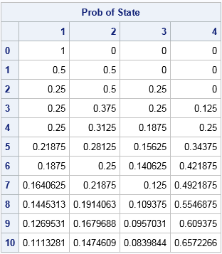
The output shows the state probabilities for a sequence of 10 coin tosses. Recall that the last row of the transition matrix ensures that the sequence stays in State 4 after it reaches State 4. Therefore the probability of the system being in State 4 is nondecreasing. The output shows that there is a 65.6% chance that the sequence HTH will appear in 10 tosses or less.

You can visualize the evolution of the probability distributions by making a series plot for each column of this output. You can download the SAS program that creates the plot and contains all of the computations in this article. The plot is shown below:

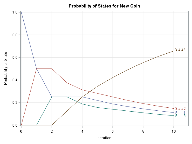
The plot shows the probability distributions after each toss when the system starts in State 1. After three time periods the system can be in any state. Over the long term, the system has a high probability of being in State 4 and a negligible chance of being in the other three states.

Modeling transitions in a population

You can also apply the transition matrix to a population of games. For example, suppose that many students are playing the game. At a certain instant, 50% of the games are in State 1, 30% are in State 2, and 20% are in State 3. You can represent that population of initial states by using the initial vector

s0 = {0.5 0.3 0.2 0};

The following graph gives the probability of the states for the population for the next 30 coin tosses:

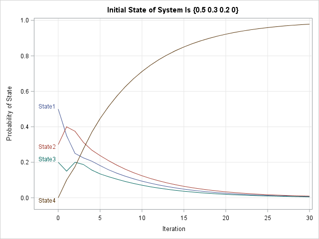
The initial portion of the graph looks different from the previous graph because the population starts in a different initial distribution of states. However, the long-term behavior of this system is the same: all games eventually end in State 4. For this initial population, the graph shows that you should expect 80% of the games to be in State 4 by the 13th toss.

A real example: Predicting caseloads for social workers and parole officers

An interesting application of using Markov chains was presented by Gongwei Chen at SAS Global Forum 2016. Chen built a discrete-time Markov chain model to forecast workloads at the Washington State Department of Corrections. Social workers and parole officers supervise convicted offenders who have been released from prison or who were sentenced to supervision by the court system. Individuals who exhibit good behavior can transition from a highly supervised situation into less supervision. Other individuals might commit a new offense that requires an increase in supervision. Chen used historical data to estimate the transition matrix between the different supervisory states. His model helps the State of Washington forecast the resources needed to supervise offenders.

Summary

In summary, it is easy to represent a transition matrix and a state vector in SAS/IML. You can iterate the initial distribution of states to forecast the state of the system after an arbitrary number of time periods. This is done by using matrix multiplication.

A Markov chain model involves iterating a linear dynamical system. The qualitative asymptotic behavior of such systems can be described by using the tools of linear algebra. In a future article, I will describe how you can compute statistical properties of Markov chain models from the transition matrix.