Visualize how parameters in a binary logistic regression model affect the probability of the event

A previous article shows that you can use the Intercept parameter to control the ratio of events to nonevents in a simulation of data from a logistic regression model. If you decrease the intercept parameter, the probability of the event decreases; if you increase the intercept parameter, the probability of the event increases.

The probability of Y=1 also depends on the slope parameters (coefficients of the regressor effects) and on the distribution of the explanatory variables. This article shows how to visualize the probability of an event as a function of the regression parameters. I show the visualization for two one-variable logistic models. For the first model, the distribution of the explanatory variable is standard normal. In the second model, the distribution is exponential.

Visualize the probability as the Intercept varies

In a previous article, I simulated data from a one-variable binary logistic model. I simulated the explanatory variable, X, from a standard normal distribution. The linear predictor is given by η = β₀ + β₁ X. The probability of the event Y=1 is given by μ = logistic(η) = 1 / (1 + exp(-η)).

In the previous article, I looked at various combinations of Intercept (β₀) and Slope (β₁) parameters. Now, let's look systematically at how the probability of Y=1 depends on the Intercept for a fixed value of Slope > 0. Most of the following program is repeated and explained in my previous post. For your convenience, it is repeated here. First, the program simulates data (N=1000) for a variable, X, from a standard normal distribution. Then it simulates a binary variable for a series of binary logistic models as the intercept parameter varies on the interval [-3, 3]. (To get better estimates of the probability of Y=1, the program simulates 100 data sets for each value of Intercept.) Lastly, the variable calls PROC FREQ to compute the proportion of simulated events (Y=1), and it plots the proportion versus the Intercept value.

/* simulate X ~ N(0,1) */
data Explanatory;
call streaminit(12345);
do i = 1 to 1000;
   x = rand("Normal",  0, 1);   /* ~ N(0,1) */
   output;
end;
drop i;
run;
 
/* as Intercept changes, how does P(Y=1) change when Slope=2? */
%let Slope = 2;
data SimLogistic;
call streaminit(54321);
set Explanatory;
do Intercept = -3 to 3 by 0.2;
   do nSim = 1 to 100;               /* Optional: param estimate is better for large samples */
      eta = Intercept + &Slope*x;    /* eta = linear predictor */
      mu = logistic(eta);            /* mu = Prob(Y=1) */
      Y = rand("Bernoulli", mu);     /* simulate binary response */
      output;
   end;
end;
run;
 
proc sort data=SimLogistic; by Intercept; run;
ods select none;
proc freq data=SimLogistic;
   by Intercept;
   tables Y / nocum;
   ods output OneWayFreqs=FreqOut;
run;
ods select all;
 
title "Percent of Y=1 in Logistic Model";
title2 "Slope=&Slope";
footnote J=L "X ~ N(0,1)";
proc sgplot data=FreqOut(where=(Y=1));
   series x=Intercept y=percent;
   xaxis grid;
   yaxis grid label="Percent of Y=1";
run;

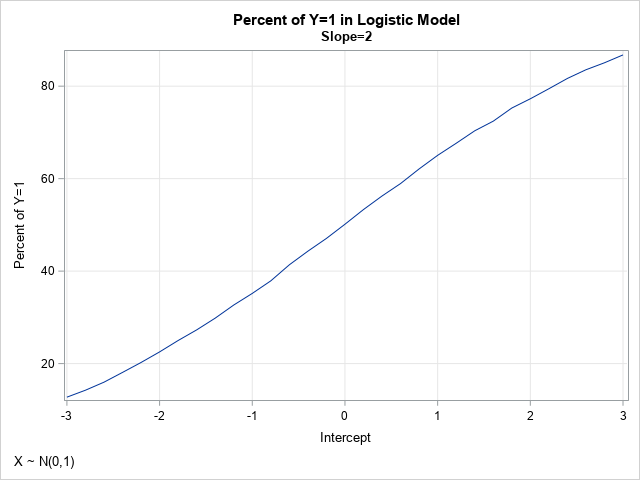
In the simulation, the slope parameter is set to Slope=2, and the Intercept parameter varies systematically between -3 and 3. The graph visualizes the probability (as a percentage) that Y=1, given various values for the Intercept parameter. This graph depends on the value of the slope parameter and on the distribution of the data. It also has random variation, due to the call to generate Y as a random Bernoulli variate. For these data, the graph shows the estimated probability of the event as a function of the Intercept parameter. When Intercept = –2, Pr(Y=1) = 22%; when Intercept = 0, Pr(Y=1) = 50%; and when Intercept = 2, Pr(Y=1) = 77%. The statement that Pr(Y=1) = 50% when Intercept=0 should be approximately true when the data is from a symmetric distribution with zero mean.

Vary the slope and intercept together

In the previous section, the slope parameter is fixed at Slope=2. What if we allow the slope to vary over a range of values? We can restrict our attention to positive slopes because logistic(η) = 1 – logistic(-η). The following program varies the Intercept parameter in the range [-3,3] and the Slope parameter in the range [0, 4].

/* now do two-parameter simulation study where slope and intercept are varied */
data SimLogistic2;
call streaminit(54321);
set Explanatory;
do Slope = 0 to 4 by 0.2;
do Intercept = -3 to 3 by 0.2;
   do nSim = 1 to 50;                  /* optional: the parameter estimate are better for larger samples */
   eta = Intercept + Slope*x;          /* eta = linear predictor */
   mu = logistic(eta);                 /* transform by inverse logit */
   Y = rand("Bernoulli", mu);          /* simulate binary response */
   output;
   end;
end;
end;
run;
 
/* Monte Carlo estimate of Pr(Y=1) for each (Int,Slope) pair */
proc sort data=SimLogistic2; by Intercept Slope; run;
ods select none;
proc freq data=SimLogistic2;
   by Intercept Slope;
   tables Y / nocum;
   ods output OneWayFreqs=FreqOut2;
run;
ods select all;

The output data set (FreqOut2) contains Monte Carlo estimates of the probability that Y=1 for each pair of (Intercept, Slope) parameters, given the distribution of the explanatory variable. You can use a contour plot to visualize the probability of the event for each combination of slope and intercept:

/* Create template for a contour plot
   https://blogs.sas.com/content/iml/2012/07/02/create-a-contour-plot-in-sas.html
*/
proc template;
define statgraph ContourPlotParm;
dynamic _X _Y _Z _TITLE _FOOTNOTE;
begingraph;
   entrytitle _TITLE;
   entryfootnote halign=left _FOOTNOTE;
   layout overlay;
      contourplotparm x=_X y=_Y z=_Z /
        contourtype=fill nhint=12  colormodel=twocolorramp name="Contour";
      continuouslegend "Contour" / title=_Z;
   endlayout;
endgraph;
end;
run;
/* render the Monte Carlo estimates as a contour plot */
proc sgrender data=Freqout2 template=ContourPlotParm;
where Y=1;
dynamic _TITLE="Percent of Y=1 in a One-Variable Logistic Model"
        _FOOTNOTE="X ~ N(0, 1)"
        _X="Intercept" _Y="Slope" _Z="Percent";
run;

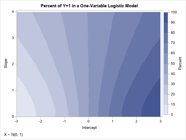
As mentioned earlier, because X is approximately symmetric, the contours of the graph have reflective symmetry. Notice that the probability that Y=1 is 50% whenever Intercept=0 for these data. Furthermore, if the points (β₀, β₁) are on the contour for Pr(Y=1)=α, then the contour for Pr(Y=1)=1-α contains points close to (-β₀, β₁). The previous line plot is equivalent to slicing the contour plot along the horizontal line Slope=2.

You can use a graph like this to simulate data that have a specified probability of Y=1. For example, if you want approximately 70% of the cases to be Y=1, you can choose any pair of (Intercept, Slope) values along that contour, such as (0.8, 0), (1, 1), (2, 3.4), and (2.4, 4). If you want to see all parameter values for which Pr(Y=1) is close to a desired value, you can use the WHERE statement in PROC PRINT. For example, the following call to PROC PRINT displays all parameter values for which the Pr(Y=1) is approximately 0.7 or 70%:

%let Target = 70;
proc print data=FreqOut2;
   where Y=1 and %sysevalf(&Target-1) <= Percent <= %sysevalf(&Target+1);
   var Intercept Slope Y Percent;
run;

Probabilities for nonsymmetric data

The symmetries in the previous graphs are a consequence of the symmetry in the data for the explanatory variable. To demonstrate how the graphs change for a nonsymmetric data distribution, you can run the same simulation study, but use data that are exponentially distributed. To eliminate possible effects due to a different mean and variance in the data, the following program standardizes the explanatory variable so that it has zero mean and unit variance.

data Expo;
call streaminit(12345);
do i = 1 to 1000;
   x = rand("Expon", 1.5);   /* ~ Exp(1.5) */
   output;
end;
drop i;
run;
 
proc stdize data=Expo method=Std out=Explanatory;
   var x;
run;

If you rerun the simulation study by using the new distribution of the explanatory variable, you obtain the following contour plot of the probability as a function of the Intercept and Slope parameters:

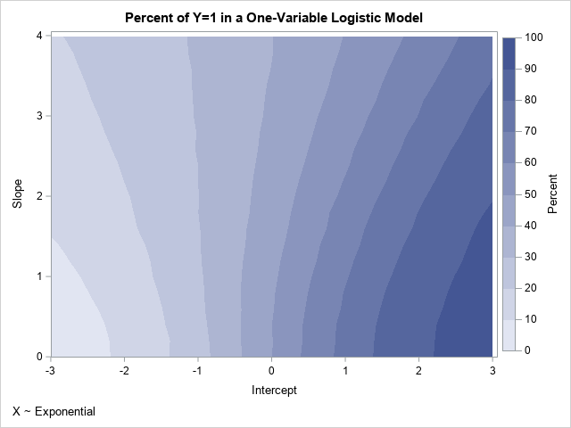
If you compare this new contour plot to the previous one, you will see that they are very similar for small values of the slope parameter. However, they are different for larger values such as Slope=2. The contours in the new plot do not show reflective symmetry about the vertical line Intercept=0. Pairs of parameters for which Pr(Y=1) is approximately 0.7 include (0.8, 0) and (1, 1), which are the same as for the previous plot, and (2.2, 3.4), and (2.6, 4), which are different from the previous example.

Summary

This article presents a Monte Carlo simulation study in SAS to compute and visualize how the Intercept and Slope parameters of a one-variable logistic model affect the probability of the event. A previous article notes that decreasing the Intercept decreases the probability. This article shows that the probability depends on both the Intercept and Slope parameters. Furthermore, the probability depends on the distribution of the explanatory variables. You can use the results of the simulation to control the proportion of events to nonevents in the simulated data.

You can download the complete SAS program that generates the results in this article.

The ideas in this article generalize to logistic regression models that contain multiple explanatory variables. For multivariate models, the effect of the Intercept parameter is similar. However, the effect of the slope parameters is more complicated, especially when the variables are correlated with each other.

Blogs