This article shows that you can use the intercept parameter to control the probability of the event in a simulation study that involves a binary logistic regression model. For simplicity, I will simulate data from a logistic regression model that involves only one explanatory variable, but the main idea applies to multivariate regression models. I also show mathematically why the intercept parameter controls the probability of the event.

The problem: Unbalance events when simulating regression data

Usually, simulation studies are based on real data. From a set of data, you run a statistical model that estimates parameters. Assuming the model fits the data, you can simulate new data by using the estimates as if they were the true parameters for the model. When you start with real data, you obtain simulated data that often have similar statistical properties.

However, sometimes you might want to simulate data for an example, and you don't have any real data to model. This is often the case on online discussion forums such as the SAS Support Community. Often, a user posts a question but cannot post the data because it is proprietary. In that case, I often simulate data to demonstrate how to use SAS to answer the question. The simulation is usually straightforward for univariate data or for data from an ordinary least squares regression model. However, the simulation can become complicated for generalized linear regression models and nonlinear models. Why? Because not every choice of parameters leads to a reasonable data set. For example, if you choose parameters "out of thin air" in an arbitrary manner, you might end up with a model for which the probability of the event (Pr(Y=1)) is close to 1 for all values of the explanatory variables. This model is not very useful.

It turns out that you can sometimes "fix" your model by decreasing the value of the intercept parameter in the model. This reduces the value of Pr(Y=1), which can lead to a more equitable and balanced distribution of the response values.

Simulate and visualize a one-variable binary logistic regression model

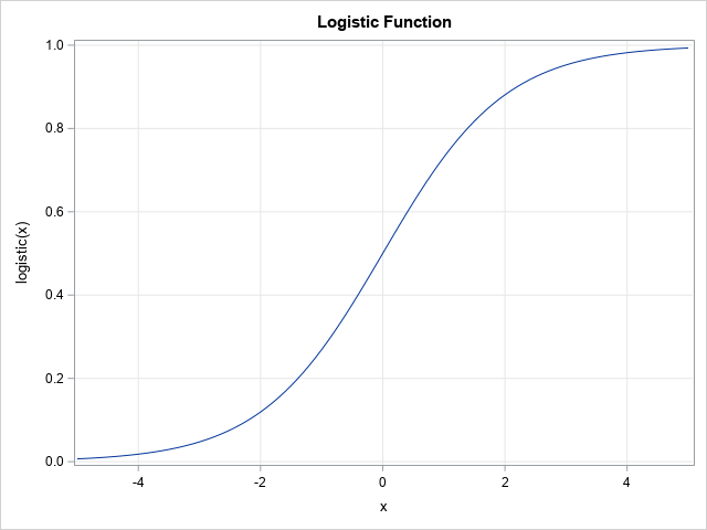
Let's construct an example. For a general discussion and a multivariate example, see the article, "Simulating data for a logistic regression model." For this article, let's keep it simple and use a one-variable model. Let X be an independent variable that is distributed as a standardized normal variate: X ~ N(0,1). Then choose an intercept parameter, β₀, and a slope parameter, β₁, and form the linear predictor η = β₀ + β₁ X. A binary logistic model uses a logistic transformation to transform the linear predictor to a probability: μ = logistic(η), where logistic(η) = 1 / (1 + exp(-η)). The graph of the S-shaped logistic function is shown to the right. You can then simulate a response as a Bernoulli random variable Y ~ Bern(μ).

In SAS, the following DATA step simulates data from a standard normal variable:

data Explanatory;
call streaminit(12345);
do i = 1 to 1000;
   x = rand("Normal",  0, 1);   /* ~ N(0,1) */
   output;
end;
drop i;
run;

Regardless of the distribution of X, the following DATA step simulates data from a logistic model that has a specified set of values for the regression parameters. I embed the program in a SAS macro so that I can run several models with different values of the Intercept and Slope parameters. The macro also runs PROC FREQ to determine the relative proportions of the binary response Y=0 and Y=1. Lastly, the macro calls PROC SGPLOT to display a graph that shows the logistic regression model and the "observed" responses as a function of the linear predictor values,

/* Simulate data from a one-variable logistic model.
   X ~ N(0,1) and Y ~ Bern(eta)
   where eta = logistic(Intercept + Slope*X).
   Display frequency table for Y and a graph of Y and Prob(Y=1) vs eta */
%macro SimLogistic(Intercept, Slope);
   title "Logistic Model for Simulated Data";
   title2 "Intercept=&Intercept; Slope=&Slope";
   data Sim1;
      call streaminit(54321);
      set Explanatory;
      eta = &Intercept + &Slope*x;   /* eta = linear predictor */
      mu = logistic(eta);            /* mu = Prob(Y=1) */
      Y = rand("Bernoulli", mu);     /* simulate binary response */
   run;
 
   proc freq data=Sim1;
      tables Y / nocum;
   run;
   proc sort data=Sim1; by eta; run;
 
   proc sgplot data=Sim1;
      label Y="Observed" mu="P(Y=1)" eta="Linear Predictor";
      scatter x=eta y=Y / transparency=0.8 markerattrs=(symbol=CircleFilled);
      series x=eta y=mu;
      xaxis grid values = (-16 to 16) valueshint;
      yaxis grid label="Probability";
      keylegend / location=inside position=E opaque;
   run;
%mend;

How does the probability of the event depend on the intercept?

Let's run the program. The following call uses an arbitrary choice of values for the regression parameters: Intercept=5 and Slope=2:

/* call the macro with Intercept=5 and Slope=2 */
%SimLogistic(5, 2);

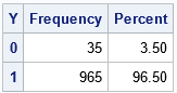
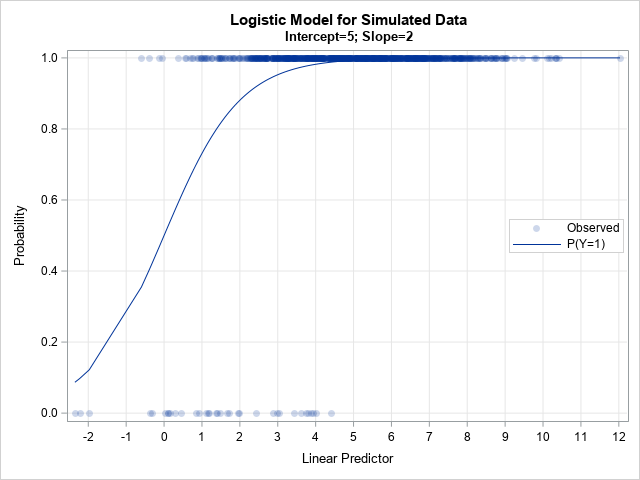
The output shows what can happen if you aren't careful when choosing the regression parameters. For this simulation, 96.5% of the response values are Y=1 and only a few are Y=0. This could be a satisfactory model for a rare event, but not for situations in which the ratio of events to nonevents is more balanced, such as 75-25, 60-40, or 50-50 ratios.

The graph shows the problem: the linear predictor (in matrix form, η = X*β) is in the range [-2, 12], and about 95% of the linear prediction are greater than 1.5. Because logistic(1.5) > 0.8, the probability of Y=1 is very high for most observations.

Since you have complete control of the parameters in the simulation, you can adjust the parameters. If you shift η to the left, the corresponding probabilities will decrease. For example, if you subtract 4 from η, then the range of η becomes [-6, 8], which should provide a more balanced distribution of the response category. The following statement implements this choice:

/* call the macro with Intercept=1 and Slope=2 */
%SimLogistic(1, 2);

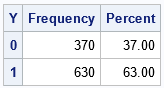
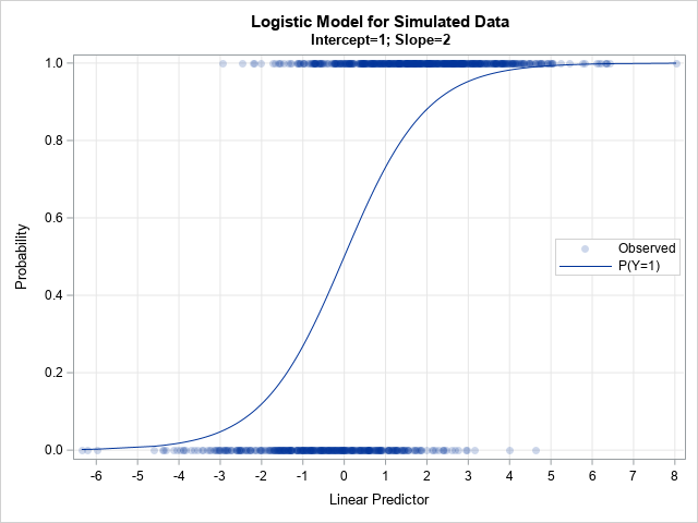
The output shows the results of the simulation after decreasing the intercept parameter. When the Intercept=1 (instead of 5), the proportion of simulated responses is more balanced. In this case, 63% of the responses are Y=1 and 37% are Y=0. If you want to further decrease the proportion of Y=1, you can decrease the Intercept parameter even more. For example, if you run %SimLogistic(-1, 2), then only 35.9% of the simulated responses are Y=1.

The mathematics

I have demonstrated that decreasing η (the linear predictor) also decreases μ (the probability of Y=1). This is really a simple mathematical consequence of the formula for the logistic function. Suppose that η₁ < η₂. Then -η₁ > -η₂
⇒    1 + exp(-η₁) > 1 + exp(-η₂) because EXP is a monotonic increasing function
⇒    1 / (1 + exp(-η₁)) < 1 / (1 + exp(-η₂)) because the reciprocal function is monotonic decreasing
⇒    μ₁ < μ₂ by definition.
Therefore, decreasing η results in decreasing μ For some reason, visualizing the simulation makes more of an impact than the math.

Summary

This article shows that by adjusting the value of the Intercept parameter in a simulation study, you can adjust the ratio of events to nonevents. Decrease the intercept parameter to decrease the number of events; increase the intercept parameter to increase the number of events. I demonstrated this fact for a one-variable model, but the main ideas apply to multivariate models for which the linear predictor (η) is a linear combination of multiple variables.

The probability of Y=1 depends continuously on the regression parameters because the linear predictor and the logistic function are both continuous. In my next article, I show how to visualize the probability of an event as a function of the regression parameters.