The area of the convex hull of random points

I recently blogged about how to compute the area of the convex hull of a set of planar points. This article discusses the expected value of the area of the convex hull for n random uniform points in the unit square. The article introduces an exact formula (due to Buchta, 1984) and uses Monte Carlo simulation to approximate the sampling distribution of the area of a convex hull. A simulation like this is useful when testing data against the null hypothesis that the points are distributed uniformly at random.

The expected value of a convex hull

Assume that you sample n points uniformly at random in the unit square, n ≥ 3. What is the expected area of the convex hull that contains the points? Christian Buchta ("Zufallspolygone in konvexen Vielecken," 1984) proved a formula for the expected value of the area of n random points in the unit square. (The unit square is sufficient: For any other rectangle, simply multiply the results for the unit square by the area of the rectangle.)

Unfortunately, Buchta's result is published in German and is behind a paywall, but the formula is given as an answer to a question on MathOverflow by 'user9072'. Let $s = \sum_{k=1}^{n+1} \frac{1}{k} (1 - \frac{1}{2^k})$ . Then the expected area of the convex hull of n points in [0,1] x [0,1] is $E[A(n)] = 1 -\frac{8}{3(n+1)} \bigl[ s - \frac{1}{(n+1)2^{n+1}} \bigr]$

The following SAS DATA step evaluates Buchta's formula for random samples of n ≤ 100. A few values are printed. You can use PROC SGPLOT to graph the expected area against n:

/* Expected area of the convex hull of a random sample of size n in the unit square.
   Result by Buchta (1984, in German), as reported by 
   https://mathoverflow.net/questions/93099/area-enclosed-by-the-convex-hull-of-a-set-of-random-points
*/
data EArea;
do n = 3 to 100;
   s = 0;
   do k = 1 to n+1;
      s + (1 - 1/2**k) / k;
   end;
   EArea = 1 - 8/3 /(n+1) * (s - 2**(-n-1) / (n+1));
   output;
end;
keep n EArea;
run;
 
proc print data=EArea noobs; 
   where n in (3,4,6,8,10,12,13) or mod(n,10)=0;
run;
 
title "Expected Area of Convex Hull";
proc sgplot data=EArea;
   series x=n y=EArea;
   xaxis grid label="Number of Random Points in Unit Square";
   yaxis grid label="Expected Area" min=0 max=1;
run;

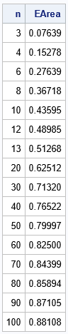
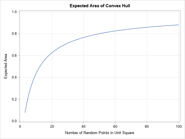
The computation shows that when n is small, the expected area, E[A(n)], is very small. The first few values are E[A(3)]=11/144, E[A(4)]=11/72, E[A(5)] = 79/360, and E[A(6)] = 199/720. For small n, the expected area increases quickly as n increases. When n = 12, the expected area is about 0.5 (half the area of the bounding square). As n gets larger, the expected area asymptotically approaches 1 very slowly. For n = 50, the expected area is 0.8. For n = 100, the expected area is 0.88.

The distribution of the expected area of a convex hull

Buchta's result gives the expected value, but the expected value is only one number. You can use Monte Carlo simulation to compute and visualize the distribution of the area statistics for random samples. The distribution enables you to estimate other quantities, such as the median area and an interval that predicts the range of the areas for 95% of random samples.

The following SAS/IML program performs a Monte Carlo simulation to approximate the sampling distribution of the area of the convex hull of a random sample in the unit square of size n = 4. The program does the following:

Load the PolyArea function, which was defined in a previous article that shows how to compute the area of a convex hull. Or you can copy/paste from that article.
Define a function (CHArea) that computes the convex hull of a set of points and returns the area.
Let B be the number of Monte Carlo samples, such as B = 10,000. Use the RANDFUN function to generate B*n random points in the unit square. This is an efficient way to generate B samples of size n.
Loop over the samples. For each sample, extract the points in the sample and call the CHArea function to compute the area.
The Monte Carlo simulation computes B sample areas. The distribution of the areas is the Monte Carlo approximation of the sampling distribution. You can compute descriptive statistics such as mean, median, and percentiles to characterize the shape of the distribution.

proc iml;
/* load the PolyArea function or copy it from 
   https://blogs.sas.com/content/iml/2022/11/02/area-perimeter-convex-hull.html
*/
load module=(PolyArea);
 
/* compute the area of the convex hull of n pts in 2-D */
start CHArea(Pts);
   indices = cvexhull(Pts);            /* compute convex hull of the N points */
   hullIdx = indices[loc(indices>0)];  /* the positive indices are on the CH */
   P = Pts[hullIdx, ];                 /* extract rows to form CH polygon */
   return PolyArea(P);                 /* return the area */
finish;
 
call randseed(1234);
NSim = 1E4;                            /* number of Monte Carlo samples */
n = 4;
X = randfun((NSim*n)//2, "Uniform");   /* matrix of uniform variates in [0,1]x[0,1] */
Area = j(NSim, 1, .);                  /* allocate array for areas */
do i = 1 to NSim;
   beginIdx = (i-1)*n + 1;             /* first obs for this sample */
   ptIdx    = beginIdx:(beginIdx+n-1); /* range of obs for this sample */
   Pts = X[ptIdx, ];                   /* use these n random points */
   Area[i] = CHArea(Pts);              /* find the area */
end;
 
meanArea = mean(Area);
medianArea = median(Area);
call qntl(CL95, Area, {0.025 0.975});
print n meanArea medianArea (CL95`)[c={LCL UCL}];

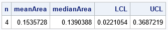
For samples of size n = 4, the computation shows that the Monte Carlo estimate of the expected area is 0.154, which is very close to the expected value (0.153). In addition, the Monte Carlo simulation enables you to estimate other quantities, such as the median area (0.139) and a 95% interval estimate for the predicted area ([0.022, 0.369]).

You can visualize the distribution of the areas by using a histogram. The following SAS/IML statements create a histogram and overlay a vertical reference line at the expected value.

title "Distribution of Areas of Convex Hull";
title2 "N=4; NSim = 10,000";
refStmt = "refline 0.15278 / axis=x lineattrs=(color=red) label='E(Area)';";
call histogram(Area) other=refStmt;

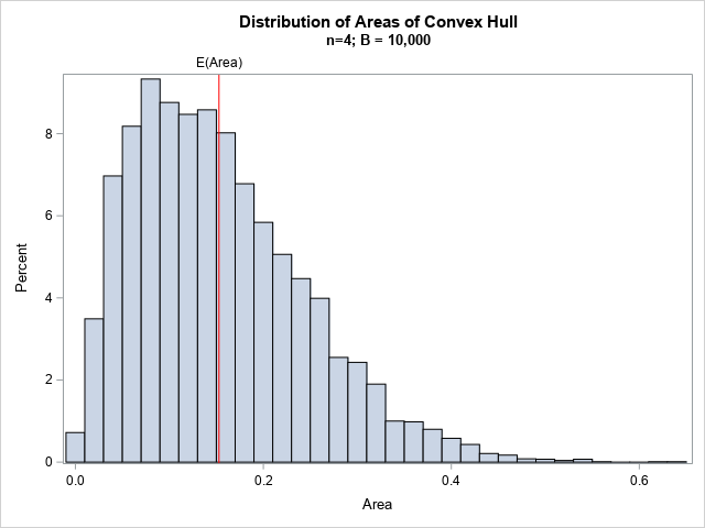
The histogram shows that the distribution of areas is skewed to the right for n = 4. For this distribution, a better measure of centrality might be the median, which is smaller than the expected value (the mean). Or you can describe the distribution by reporting a percentile range such as the inter-quartile range or the range for 95% of the areas.

Graphs of the distribution of the area of a convex hull

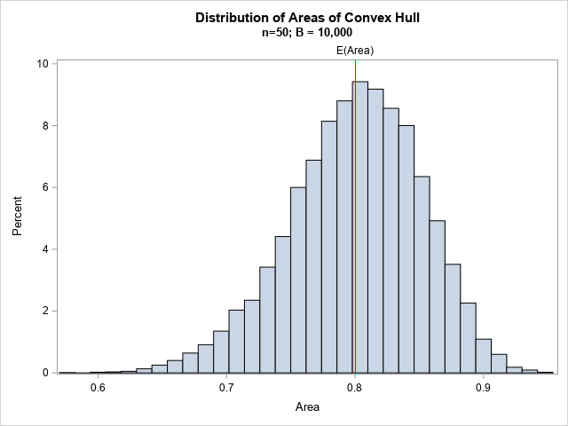
You can repeat the previous Monte Carlo simulation for other values of n. For example, if you use n = 50, you get the histogram shown to the right. The distribution for n = 50 is skewed to the left. A prediction interval for 95% of areas is [0.69, 0.89].

Whether or not you know about Buchta's theoretical result, you can use Monte Carlo simulation to estimate the expected value for any sample size. The following SAS/IML program simulates 10,000 random samples of size n for n in the range [3, 100]. For each simulation, the program writes the estimate of the mean and a prediction interval to a SAS data set. You can use the BAND statement in PROC SGPLOT to overlay the interval estimates and the estimate of the expected value for each value of n:

/* repeat Monte Carlo simulation for many values of N. Write results to a data set and visualize */
create ConvexHull var {'n' MeanArea LCL UCL};
 
numPts = 3:100;
NSim = 1E4;                            /* number of Monte Carlo samples */
do j = 1 to ncol(numPts);                 /* number of random pts for each convex hull */
   N = numPts[j];
   X = randfun((NSim*N)//2, "Uniform");   /* matrix of uniform variates in [0,1]x[0,1] */
   Area = j(NSim, 1, .);                  /* allocate array for areas */
   LCL = j(NSim, 1, .);                   /* allocate arrays for 95% lower/upper CL */
   UCL = j(NSim, 1, .);
   do i = 1 to NSim;
      beginIdx = (i-1)*N + 1;             /* first obs for this sample */
      ptIdx    = beginIdx:(beginIdx+N-1); /* range of obs for this sample */
      Pts = X[ptIdx, ];                   /* use these N random points */
      Area[i] = CHArea(Pts);
   end;
 
   meanArea = mean(Area);
   call qntl(CL95, Area, {0.025 0.975});
   LCL = CL95[1];   UCL = CL95[2];
   append;
end;
close ConvexHull;
QUIT;
 
title "Monte Carlo Estimate of Expected Area of Convex Hull";
proc sgplot data=ConvexHull noautolegend;
   band x=n lower=LCL upper=UCL / legendlabel="95% Prediction";
   series x=n y=meanArea / legendlabel="Expected Area";
   keylegend / location=inside position=E opaque across=1;
   xaxis grid label="Number of Random Points in Unit Square";
   yaxis grid label="Expected Area" min=0 max=1;
run;

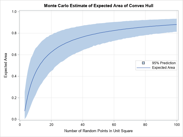
From this graph, you can determine the expected value and a 95% prediction range for any sample size, 3 ≤ n ≤ 100. Notice that the solid line is the Monte Carlo estimate of the expected value. This estimate is very close to the true expected value, which we know from Buchta's formula.

Summary

Some researchers use the area of a convex hull to estimate the area in which an event occurs. The researcher might want to test whether the area is significantly different from the area of the convex hull of a random point pattern. This article presents several properties of the area of the convex hull of a random sample in the unit square. The expected value of the area is known theoretically (Buchta, 1984). Other properties can be estimated by using a Monte Carlo simulation.

You can download the SAS program that generates the tables and graphs in this article.

Blogs