A SAS programmer asked how to create a graph that shows whether missing values in one variable are associated with certain values of another variable. For example, a patient who is supposed to monitor his blood glucose daily might have more missing measurements near holidays and in the summer months due to vacations. In this example, the "missingness" in the glucose variable is related to the date variable. In general, we say that missing values depend on another variable when the probability of obtaining a missing value in one variable depends on the value of another variable.

It can be useful to visualize the dependency if you are trying to impute values to replace the missing values. In missing-value imputation, the analyst must decide how to model the missing values. Three popular assumptions are that the values are missing completely at random (MCAR), missing at random (MAR), or missing not at random (MNAR). You can read more about these missing-value assumptions. The visualization in this article can help you decide whether to treat the data as MCAR or MAR.

Generate fake data and missing values

Let's generate some fake data. The following DATA step creates four variables:

• The DATE variable does not contain any missing values. It contains daily values between 01JAN2018 and 31DEC2020.
• The X1 variable is missing only in 2020. In 2020, there is an 8% probability that X1 is missing.
• The X2 variable is missing only on Sundays. On Sundays, there is a 10% probability that X2 is missing.
• The X3 variable is nonmissing from March through October. During the winter months, there is a 5% probability that X3 is missing.

/* generate FAKE data to use as an example */
data Have;
call streaminit(1234);
format Date DATE9.;
do Date = '01JAN2018'd to '31DEC2020'd;
   x1 = rand("Normal");
   x2 = rand("Normal");
   x3 = rand("Normal");
   /* assign missing values:
      x1 is missing only in 2020
      x2 is missing only on Sundays
      x3 is missing only in Nov, Dec, Jan, and Feb
   */
   if year(Date)=2020            & rand("Bernoulli", 0.08) then x1 = .;
   if weekday(date)=1            & rand("Bernoulli", 0.10) then x2 = .;
   if month(date) in (11,12,1,2) & rand("Bernoulli", 0.05) then x3 = .;
   output;
end;
run;

The goal of this article is to create a graph that indicates how the missing values in the X1-X3 variables depend on time. In a previous article, I showed how to use heat maps in SAS/IML to visualize missing values. In the next section, I use the SAS DATA step to transform the data into a form that you can visualize by using the HEATMAPPARM statement in PROC SGPLOT.

Visualize patterns of missing values

To visualize the patterns of missing values, I use the following ideas:

• Filter the data to keep only observations that have missing values. This is the opposite of the usual "listwise deletion" operation in which we keep only complete cases.
• Convert the data from wide format to long format. Create new variables, VARNAME and ISMISSING. The variable VARNAME contains the names of the original variables: "X1", "X2", and "X3." The variable ISMISSING is a binary indicator variable that indicates whether the variable has a missing value for a given date.
• Create a heat map in that shows the missing values for each variable for each date. For consistency, I create a discrete attribute map that ensures that the heat map displays missing values in black and nonmissing values in white.

/* Plot missing values of X1-X3 versus the values of Date. */
%let IndepVar = Date;           /* variable to show on Y axis */
%let DepVars  = x1 x2 x3;       /* visualize missing values for these variables */
 
/* 1. Filter the data to keep only observations that have missing values.
   2. Convert from wide to long. New variables VARNAME and ISMISSING contain the 
      information to plot.   */
data Want;
set Have;
length varName $32;
array xVars[3] &DepVars;        /* response variables (inputs) */
ObsNum = _N_;                   /* if you want the original row number */
if nmiss(of xVars[*]) > 0;      /* keep only obs that have missing values */
do i = 1 to dim(xVars);
   varName = vname(xVars[i]);   /* assign the name of the original variable */
   isMissing = nmiss(xVars[i]); /* binary indicator variable */
   output;
end;
keep ObsNum &IndepVar varName isMissing;
run;
 
/* 3. Define discrete attribute map: missing values are black and nonmissing values are white. */
data AttrMap;
  retain id 'HeatMiss';
  length fillcolor $20;
  value=0; fillcolor='White'; output;  /* nonmissing = white */
  value=1; fillcolor='Black'; output;  /* missing = black */
run;
 
/* 4. Create a heat map that shows the missing values for each variable for each date. */
/*    Thanks to Dan Heath for suggesting that I use INTERVAL=QUARTER
      for major ticks and MINORINTERVAL=MONTH for minor ticks */
ods graphics / width=400px height=600px;
title "Visualize Missing Values";
proc sgplot data=Want dattrmap=AttrMap;
   heatmapparm x=varName y=&IndepVar colorgroup=isMissing / attrid=HeatMiss;
   xaxis display=(nolabel);
   yaxis display=(nolabel) type=time interval=quarter valuesformat=monyy7. 
                           minor minorinterval=month;
run;

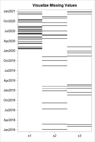
The heat map is shown to the right. It displays dates along the vertical axis. The horizontal axis displays the three numerical variables that have missing values. You can use the graph to determine whether the pattern of missing values depend on the Date variable. In the program, I used macro variables to store the name of the X and Y variables so that the program is easier to reuse.

What does the heat map show?

• For the X1 variable, the heat map clearly shows that the variable does not have any missing values prior to 2020, but then has quite a few in 2020. The graph is consistent with the fact that the missing values in 2020 are distributed uniformly. You can see gaps and clusters, which are common features of uniform randomness.
• For the X2 variable, the heat map is less clear. It is possible that the missingness occurs uniformly at random for any date. You would need to run an additional analysis to discover that all the missing values occur on Sundays.
• For the X3 variable, the heat map suggests that the missing values occur in the winter months. However, you should probably run an additional analysis to discover that all the missing values occur between November and February.

You can use PROC FREQ to perform additional analyses on the X2 and X3 variables. The following calls to PROC FREQ use the MONTHw. and WEEKDAYw. formats to format the Date variable. PROC FREQ can perform a two-way analysis to investigate whether missingness in X2 and X3 is associated with days or months, respectively. You can use a mosaic plot to show the results, as follows:

ods graphics / reset;
proc freq data=Want order=formatted;
   where varName="x2";
   format Date WEEKDAY.;
   label IsMissing = "Missing Value for X2" Date = "Day of Week";
   tables IsMissing * Date / plots=MosaicPlot;
run;
 
proc freq data=Want order=formatted;
   where varName="x3";
   format Date MONTH.;
   label IsMissing = "Missing Value for X3" Date = "Month of Year";
   tables IsMissing * Date / plots=MosaicPlot;
run;

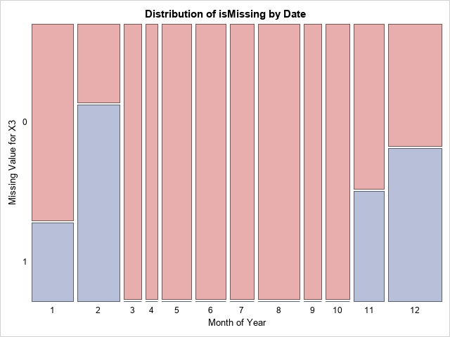
For brevity, only the mosaic plot for the month of the year is shown. The mosaic plot shows that all the missing values for X3 occur in November through February. A similar plot shows that the missing values for X2 occur on Sunday.

Summary

This article shows how to use a heat map to plot patterns of missing values for several variables versus a date. By plotting the missing values of X1, X2, X3,..., you can assess whether the missing values depend on time. This can help you to decide whether the missing values occur completely at random (MCAR). The missing values in this article are not MCAR. However, that fact is not always evident from the missing value pattern plot, and you might need to run additional analyses on the missing values.

Although this analysis used a date as the independent variable, that is not required. You can perform similar visualizations for other choices of an independent variable.