For some reason, SAS programmers like to express their love by writing SAS programs. Since Valentine's Day is next week, I thought I would add another SAS graphic to the collection of ways to use SAS to express your love.

Last week, I showed how to use vector operation and a root-finding algorithm to visualize the path of a ball rolling on an elliptical billiards table. Every time the ball hits the boundary of the table, it rebounds and continues rolling in a new direction. At the end of the article, I commented that "the same program can compute the path of a ball on any table" for which certain conditions hold. With Valentine's Day coming soon, I wondered whether I could visualize the dynamics of a ball bouncing across a heart-shaped table. The graph to the right is the result of my efforts.

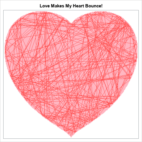
In the figure, the pink area is the interior of the heart-shaped billiard table. The red lines trace the path of a ball that starts in the middle of the heart with an initial motion at 45 degrees to the horizontal. The figure shows the ball's path for the first 250 bounces.

Although the caption of the figure is "Love Makes My Heart Bounce," the figure might also resonate with people who feel like they bounce around and never find love. It might appeal to those who have recently ended a relationship and feel like they are on the rebound. And during the global pandemic, maybe you have stayed close to home, never venturing very far from those you love? This heart is for you, too!

Details of the computation

Here are a few details about the computation:

• The shape of the heart is defined by $H(x,y)=0$, where $H(x,y) = (x^2 + y^2 - 1)^3 - x^2 y^3$.
• The gradient of H vanishes at the four points on the curve, namely (0, ±1) and (±1, 0). If the virtual ball "hits" the table's virtual boundary at those locations, the ball will "stick" to the boundary because the program uses the gradient of the function to compute the normal vector to the curve. The program could be modified to compute the normal vector at (±1, 0). However, the curve has a cusp singularity at (0, ±1), so it is impossible to define a normal vector at those points. On a real billiard table, you would want to round off the singularity at those points.
• Because the heart shape is not convex, I had to modify the routine that finds the intersection of a ray and the curve H=0. The previous article on this topic assumes that a ray intersects the curve at only one point. Along the top of the heart, a ray might intersect the curve at three points. I modified the program to find the nearest intersection point.

You can download the program that I used to make the graph. Feel free to change the colors and caption and spread the love.