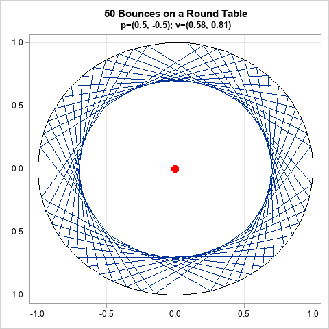
I recently showed how to find the intersection between a line and a circle. While working on the problem, I was reminded of a fun mathematical game. Suppose you make a billiard table in the shape of a circle or an ellipse. What is the path for a ball at position p on the table if it rolls in a specified direction, as determined by a vector, v? A possible path is shown in the graph at the right for a circular table. The figure shows the first 50 bounces for a ball that starts at position p=(0.5 -0.5) and travels in the direction of v=(1, 1).
This article shows how to use SAS to compute images like this for circular and elliptical tables.
Vectors and geometry
One of the advantages of the SAS/IML matrix language is its natural syntax: You can often translate an algorithm from its mathematical formulation to a computer program by using only a few statements. This section presents the mathematical formulation for finding the trajectories of a ball on a circular or elliptical billiard table, then shows how to translate the math into SAS/IML statements.
The fundamental mathematical assumption is that all collisions are perfectly elastic and that the angle of incidence equals the angle of reflection. For a curved surface, the angles are measured by using the normal and tangent vectors to the curve. The geometry is shown in the following figure.
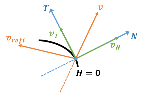
A ball moves toward the boundary of the table with velocity vector v. The boundary is represented as the level set H = 0 for some bivariate function, H(x). For example, a circular table uses H(x,y) = x2 + y2 - 1. The previous article showed how to find the point at which the ball hits the curve.
You can compute the unit normal vector, N, at that point by using the gradient of H. Project the velocity vector onto the unit normal to obtain vN. The linear space orthogonal to N is the tangent space. The vector vT = v - vN is the projection of v onto the tangent space. (Note that v = vT + vN.) The reflection of v is defined to be the vector that has the same tangent components but the opposite normal components, which is vrefl = vT - vN. A little algebra shows that vrefl = v - 2vN, so, in practice, the projection onto the tangent space is not needed.
The following SAS/IML program implements functions that compute these vectors. To test the functions, assume a ball is initially at the point p=(0.5, -0.5) and moves with unit velocity v=(1, 1)/sqrt(2), which is 45 degrees from the horizontal.
proc iml; /* Define the multivariate function H and its gradient. Example: H(x)=0 defines a circle and grad(H) is the gradient */ start H(x); return( x[ ,1]##2 + x[ ,2]##2 - 1 ); /* = x##2 + y##2 - 1 */ finish; start gradH(x); return( 2*x ); /* { dH/dx dH/dy } */ finish; /* given x such that H(x)=0 and a unit vector, v, find the normal and tangent components of v such that v = v_N + v_T, where v_N is normal to H=0 and v_T is tangent to H=0 */ /* project v onto the normal space at x */ start NormalH(x, v); grad = gradH(x); /* if H(x)=0, grad(H) is normal to H=0 at x */ N = grad / norm(grad);/* unit normal vector to curve at x */ v_N = (v*N`) * N; /* projection of v onto normal vetor */ return( v_N ); finish; /* project v onto the tangent space at x */ start TangentH(x, v); v_N = NormalH(x, v); v_T = v - v_N; return( v_T ); finish; /* reflect v across tangent space at x */ start Reflect(x, v); v_N = NormalH(x, v); v_refl = v - 2*v_N; return( v_refl ); finish; /* Test the definitions for the following points and direction vector */ p = {0.5 -0.5}; /* initial position of ball */ v = {1 1} / sqrt(2); /* unit velocity vector: sqrt(2) = 0.7071068 */ q = {1 0}; /* ball hits circle at this point */ N = NormalH(q, v); /* normal component to curve at q */ T = TangentH(q, v); /* tangential component to curve at q */ v_refl = Reflect(q, v); /* reflection of v */ print v, N, T, v_refl; |
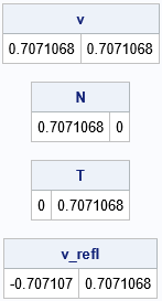
From the initial position and velocity, it is clear that the ball will hit the circle at q=(1,0) and reflect off at 135 degrees, which is the direction vector vrefl=(-1, 1)/sqrt(2). For this geometry, the unit normal vector at q is N=(1,0) and the unit tangent vector is T=(0,1), so it is easy to mentally verify that the program is giving the correct values for the vectors in this problem.
Bouncing around a billiard table
Let's play a game of billiards on a table that has a nonstandard shape. To begin the game, you must specify the initial position (p) and velocity (v) of the ball, as well as the shape of the table (a function H). The algorithm is simple:
- Given p and v, find the point q where the ball hits the boundary of the table. This step is described in a previous article..
- Reflect v across the normal vector at q to obtain a new direction, vrefl.
- Repeat this process some number of times. Optionally, plot the path to visualize how the ball bounces across the table.
The following SAS/IML program implements this algorithm by using the F_Line and FindIntersection functions from the previous article:
/* To find the intersection of H=0 with the line through G_p in the direction of G_v, see https://blogs.sas.com/content/iml/2022/02/02/line-search-sas.html */ /* Restriction of H to the line through G_p in the direction of G_v */ start F_Line(t) global(G_p, G_v); return( H( G_p + t*G_v ) ); finish; /* return the intersection of H=0 and the line */ start FindIntersection(p, v, step=20) global(G_p, G_v); G_p = p; G_v = v; t = froot("F_Line", 1E-3 || step); /* find F(t) = 0 for t in [1E-3, step] */ q = p + t*v; /* H(q) = 0 */ return( q ); finish; /* given a point, p, and a direction vector, v, find the point q on the line through p in the direction of v such that H(q)=0. Reflect the velocity vector to get a new direction vector, v_refl */ start HitTable(q, v_refl, p, v); q = FindIntersection(p, v); v_refl = Reflect(q, v); finish; /* Example: A periodic path with four segments */ p = {0.5 -0.5}; /* point p */ v = {1 1}/sqrt(2); /* direction vector v */ NSeg = 6; /* follow for this many bounces */ x = j(NSeg, ncol(p)); x[1,] = p; do i = 2 to NSeg; run HitTable( q, v, x[i-1,], v ); /* overwrite v on each iteration */ x[i,] = q; end; print x[L="Positions"]; |
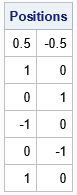
These initial conditions are highly symmetric and therefore easy to visualize. From the initial position and velocity, the ball hits the boundary of the circular table at (1,0), (0,1), (-1,0), and (0,-1) before returning again to (1,0). The ball will follow this periodic trajectory forever. It will always hit the same four points on the boundary of the circle.
For a general initial condition, you will want to draw a graph that visualizes the orbit of the ball as it bounces across the table. You can download the SAS program that computes the graphs in this article. For ease of use, I encapsulated the computations and visualization into a module called Billiards. You can call the Billiards subroutine with an initial condition and the number of bounces and the module will return a graph of the trajectory of the ball. For example, the following statements generate the first 50 bounces of a ball on a circular table:
/* Example 2. Either periodic orbit or bounces inside an annulus */ p = {0.5 -0.5}; /* point p */ v = {1 1.4}; /* vector v */ v = v / norm(v); /* standardize to unit vector */ print v; title "50 Bounces on a Round Table"; title2 "p=(0.5, -0.5); v=(0.58, 0.81)"; run Billiards(p, v, 50); /* NSeg=50 bounces */ |
The graph is shown at the top of this article. For this example, the ball bounces around the table inside an annular region. For a circular table, you can prove mathematically that every trajectory is either a periodic orbit or is dense in an annular region.
Billiards on an elliptical table
If you study the previous program, you will see that the program does not use any special knowledge of the shape of the table. Given any smooth functions H and grad(H), the program should be able to handle tables of other shapes. That is the advantage of writing a program that uses vectors in a coordinate-free manner.
Let's change the functions for H and grad(H) to use an elliptical table with parameters a and b. That is, the shape of the table is determined by H(x)=0, where \(H(\mathbf{x}) = x_1^2/a^2 + x_2^2/b^2 - 1\) is the standard form of an ellipse. For the next example, let's use a=sqrt(5) and b=2.
/* define the elliptical region and gradient vector */ start H(x); a = sqrt(5); b = 2; return( (x[ ,1]/a)##2 + (x[ ,2]/b)##2 - 1 ); /* ellipse(a,b) */ finish; start gradH(x); a = sqrt(5); b = 2; return( 2*x[ ,1]/a##2 || 2*x[ ,2]/b##2 ); finish; |
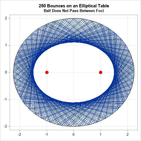
An ellipse is determined by its two foci, which are located at (+/-sqrt(a2 - b2), 0) when a > b. For our example, the foci are at (-1, 0) and (1, 0).
You can show that the path of a ball on an elliptical table is one of three shapes:
- If the ball does not pass between the foci, its path is inside an annular region.
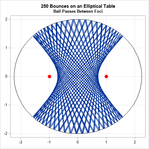
- If the ball passes between the foci, its path is inside a hyperbolic region.
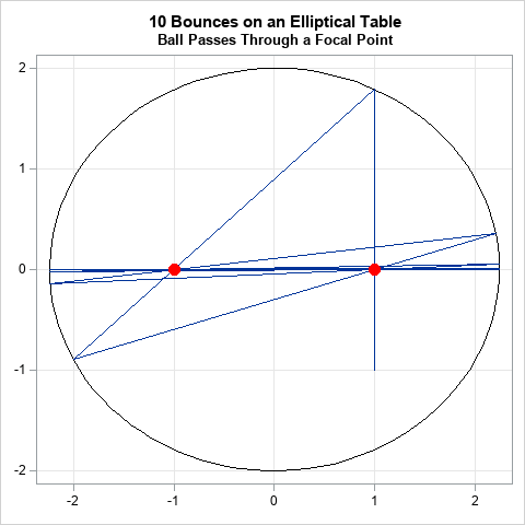
- If the ball passes over one focal point, it also passes over the second focal point. The path converges to the major axis that contains the foci.
The following examples show each case:
/* If the ball does not pass between the foci, its path is inside an annular region. */ p = {1.5 0}; /* point p */ v = {0 1}; /* vector v */ title "250 Bounces on an Elliptical Table"; title2 "Ball Does Not Pass Between Foci"; run Billiards(p, v, 250); |
/* If the ball passes between the foci, its path is inside a hyperbolic region. */ p = {0 0}; /* point p */ v = {1 1}/sqrt(2); /* vector v */ title "250 Bounces on an Elliptical Table"; title2 "Ball Passes Between Foci"; run Billiards(p, v, 250); |
/* If the ball passes over one focal point, it also passes over the second focal point. The path converges to the major axis that contains the foci. */ p = {1 -1}; /* point p */ v = {0 1}; /* vector v */ title "10 Bounces on an Elliptical Table"; title2 "Ball Passes Through a Focal Point"; run Billiards(p, v, 10); |
Summary
In summary, you can use analytical geometry to figure out the trajectory of a ball on nonstandard billiard table that has a curved boundary. By using vectors and a root-finding algorithm in the SAS/IML language, you can write a program that displays the path of a ball on a circular table. The advantage of a coordinate-free vector formulation is that the same program can compute the path of a ball on a table that has a more complicated boundary, such as an ellipse. In fact, the same program can compute the path of a ball on any table for which H=0 defines a smooth convex curve on which the gradient of H does not vanish.
Incidentally, people have built elliptical billiard tables and have put a hole at one of the foci. To sink a ball, you can shoot it at the hole or you can shoot it at the other focal point. Either way, the ball rolls into the hole.
You can download the SAS program that I used to create the graphs in this article.

1 Comment
Pingback: Billiards on a heart-shaped table - The DO Loop