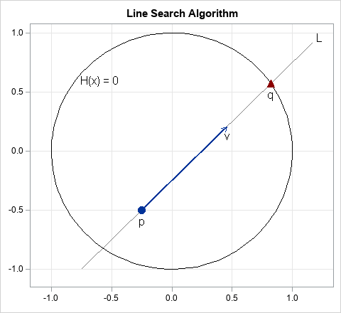
Recently, I needed to implement a line search algorithm in SAS. The line search is illustrated by the figure at the right. You start with a point, p, in d-dimensional space and a direction vector, v. (In the figure, d=2, but in general d > 1.) The goal is to search along the line, L, that passes through p in the direction of v. Typically, you are searching for the root of some scalar-valued multivariate function, H(x). The goal is to search along the line until you intersect the curve given by H(x)=0. In the figure, \(H(\mathbf{x}) = x_1^2 + x_2^2 - 1\), so the expression H(x)=0 defines the unit circle, where x = (x1, x2). In the figure, the search finds the point q, which is on the unit circle. This point might not be unique. In general, the line might intersect the curve H(x)=0 at multiple points, or not at all. For this example, the line intersects the circle at two points.
The quantities in the figure are d-dimensional, yet the line search enables you to perform a one-dimensional search along a line. Along the line, the coordinates are given by the vector expression x = p + t v, for any real value of the parameter t. The line search turns a d-dimensional problem into a one-dimensional problem: Find the root of the function F(t) = H(p + t v).
This article shows how to implement a line search algorithm in SAS by using the SAS/IML language. When you use a matrix language, the program is amazingly compact.
A line search algorithm
You can implement the line search algorithm in four steps:
- Define the multivariate function H(x). The search will find a point x such that H(x) = 0.
- Define the point, p, and vector, v. These define a line whose parametric form is p + t*v for real values t. The vector v is often standardized to create a unit vector, but that is not necessary.
- Define an objective function F(t) = H(p + t v), which is the restriction of H to the line.
- Find a root of the function F. This provides a value t=T such that F(T) = 0. This means that the point q = H(p + T v) satisfies H(q) = 0.
One of the advantages of the SAS/IML matrix language is that you can often directly translate an algorithm from its mathematical formulation to its syntax in a natural way. The following program implements the line search algorithm:
proc iml; /* 1. Define the multivariate function H. Goal: find a point such that H(x)=0. */ start H(x); /* if x is 2D point, H=0 is a circle */ return ( x[ ,##] - 1 ); /* return x##2 + y##2 - 1; the '##' operator is sum of squares */ finish; /* 2. Define the point, p, and vector, v. These will be used as parameters for a root-finding algorithm, so make them GLOBAL variables. */ G_p = {-0.25 -0.5}; /* point p */ v = {1 1}; /* vector v */ G_v = v / norm(v); /* optional: standardize to unit vector */ /* 3. Define an objective function, F(t), which is the restriction of H to a line. */ start F_Line(t) global(G_p, G_v); return ( H( G_p + t*G_v ) ); finish; /* 4. Call the FROOT function to find a root of the function F. */ t = froot("F_Line", {0 2}); /* find t such that F(t) = 0 */ q = G_p + t*G_v; /* find q such that H(q) = 0 */ print q, t (H(q))[L="H(q)"]; |
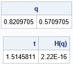
The program is quite compact. Each step requires only a few lines to implement. The result is that the point (0.82, 0.57) is a point on the unit circle. It is one of the points that lies on the line with unit slope that passes through the point (-0.25, -0.5).
In this implementation, there are three IML-specific statements that I want to explain:
- The expression x[ ,##] means "for each row of the matrix x, compute the sum of the squares of the elements in each column." The '##' operator is an example of a subscript reduction operator.
- You can use the GLOBAL statement to pass parameters to a function for which you want to find the root. The argument to the function (t) is varied during the root-finding algorithm whereas the GLOBAL parameters are held constant.
- The FROOT function finds the root of a function of one variable. It assumes that the graph of the function along the line is transverse at the root. That is, the function is positive on one side of the root and negative on the other side.
More solutions along the line
As mentioned previously, there are two points along the line that intersect the unit circle. You can get the other point by searching in the direction of -v or by considering negative values for the parameter t. I prefer the second method. The second argument to the FROOT function is a matrix of intervals to search for a root. The following statement finds two roots for F(t), one in the interval [0, 2] and the other in the interval [-2, 0].
/* There is also a solution in direction of negative t. */ t = froot("F_Line", {-2 0, /* search for t in interval [-2, 0] */ 0 2}); /* also search in interval [0, 2] */ q = G_p + t*G_v; print q, t (H(q))[L="H(q)"]; |
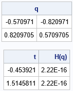
The output shows that the point (-0.57, -0.82) is another point of intersection between the circle and the line.
Generalizing to higher dimensions
Here's an interesting question to consider. The previous program solves the case of a line intersecting the unit circle in the 2-D plane. How much of the program do you need to change to solve the generalized problem of a line intersecting a unit sphere in 3-D space? If you want to ponder that question, stop reading and study the program carefully before you read on.
Ready? Okay. The answer is that you don't have to change any of the computational statements in the program. None. Zero. Zip. Zilch. Nada. I wrote the program by using a coordinate-free vector formulation. Consequently, the same functions work for a line search in higher dimensions. For example, the following program finds the intersections of a line in 3-D space and the unit sphere. The line is defined by specifying a 3-D point and a 3-D vector, which determines a direction:
G_p = {-0.25 -0.5 0.1}; /* point in 3-D space */ G_v = {1 1 1}; /* vector in 3-D space */ t = froot("F_Line", {-2 0, /* search for t in interval [-2, 0] */ 0 2}); /* also search in interval [0, 2] */ q = G_p + t*G_v; print q; |
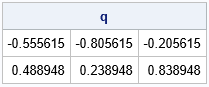
The output tells you that the line intersects the sphere at two points: q1 = (-0.56, -0.81, -0.21) and q2 = (0.49, 0.24, 0.84). The computational portions of the program are independent of the dimensions of the space. Of course, if you want to intersect a surface that is different than the unit sphere, you will have to redefine the function that evaluates the H function, but you would not have to change the F function.
Summary
In summary, this article shows how to implement a line search algorithm in SAS by using the SAS/IML language. The implementation in a matrix language is very compact. Furthermore, it is often the case that key portions of the program can be written in a coordinate-free manner, which means that the program can be easily modified to handle line searches in arbitrary dimensions.
