While discussing how to compute convex hulls in SAS with a colleague, we wondered how the size of the convex hull compares to the size of the sample. For most distributions of points, I claimed that the size of the convex hull is much less than the size of the original sample. This article looks at the expected value of the proportion p = k / N, where k is the size of the convex hull for a set of N planar points. The proportion depends on the distribution of the points. This article shows the results for three two-dimensional distributions: the uniform distribution on a rectangle, the normal distribution, and the uniform distribution on a disk.

Monte Carlo estimates of the expected number of points on a convex hull

You can use Monte Carlo simulation to estimate the expected number of points on a convex hull. First, specify the distribution of the points and the size of the sample, N. Then do the following:

• Simulate N random points from the distribution and compute the convex hull of these points. This gives you a value, k, for this one sample.
• Repeat the simulation B times. You will have B values of k: {k₁, k₂, ..., k_B}.
• The average of the B values is an estimate of the expected value for the number of points on the convex hull for a random set of size N.
• If you prefer to think in terms of proportions, the ratio k / N is an estimate of the expected proportion of points on the convex hull.

Simulate uniform random samples for N=200

Before you run a full simulation study, you should always run a smaller simulation to ensure that your implementation is correct. The following SAS/IML statements generate 1000 samples of size N=200 from the uniform distribution on the unit square. For each sample, you can compute the number of points on the convex hull. You can then plot the distribution of the number of points on the convex hull, as follows:

proc iml;
call randseed(1);
 
/* 1. Convex hull of N=200 random uniformly distributed 
      points in the unit square [0,1] x [0,1] */
NRep = 1000;            /* number of Monte Carlo samples */
Distrib = "Uniform";
N = 200;                /* sample size */
k = j(NRep, 1, 0);      /* store the number of points on CH */
X = j(N, 2, 0);         /* allocate matrix for sample */
do j = 1 to NRep;
   call randgen(X, Distrib);  /* random sample */
   Indices = cvexhull(X);
   k[j] = sum(Indices>0);     /* the positive indices are on CH */
end;
 
Ek = mean(k);           /* MC estimate of expected value */
print Ek;
title "k = Number of Points on Convex Hull; N = 200";
call bar(k) other="inset ('E[k] =' = '13.88') / border;";

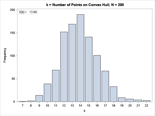
The bar chart shows the distribution of the size of the convex hull for the 1,000 simulated samples. For most samples, the convex hull contains between 12 and 15 points. The expected value is the average of these values, which is 13.88 for this simulation.

If you want to compare samples of different sizes, it is useful to standardize the estimated quantity. Rather than predict the number of points on the convex hull, it is useful to predict the proportion of the sample that lies on the convex hull. Furthermore, we should report not only the expected value but also a confidence interval. This makes it clearer that the proportion for any one sample is likely to be within a range of values:

p = k / N;              /* proportion of points on the CH */
mean = mean(p);         /* expected proportion */
call qntl(CI, p, {0.025, 0.975}); /* 95% confidence interval */
print mean CI;
 
refStmt = 'refline ' + char(mean//CI) + '/ axis=X lineattrs=(color=red);';
title "Proportion of Points on Convex Hull, 1000 Random Samples";
title2 "X ~ U(Square); N = 200";
call histogram(p) other=refStmt label='Proportion';

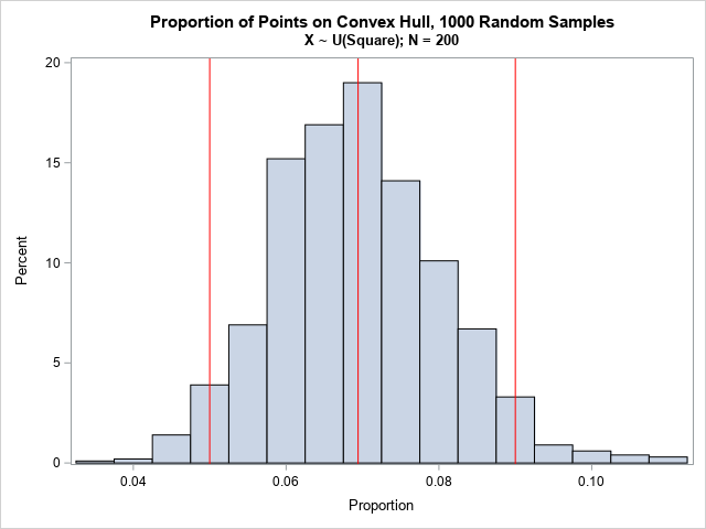
For this distribution of points, you should expect about 7% of the sample to lie on the convex hull. An empirical 95% confidence interval is between 5% and 9%.

According to an unpublished preprint by Har-Peled ("On the Expected Complexity of Random Convex Hulls", 2011), the asymptotic formula for the expected number of points on the convex hull of the unit square is O(log(n)).

Simulate samples for many sizes

The previous section simulated B samples for size N=200. This section repeats the simulation for values of N between 300 and 8,000. Instead of plotting histograms, I plot the expected value and a 95% confidence interval for each value of N. So that the simulation runs more quickly, I have set B=250. The following SAS/IML program simulates B samples for various values of N, all drawn from the uniform distribution on the unit square:

/* 2. simulation for X ~  U(Square), N = 300..8000 */
NRep = 250;  /* Monte Carlo simulation: use 250 samples of size N */
Distrib = "Uniform";
N = do(300, 900, 100) || do(1000, 8000, 500);  /* sample sizes */
k = j(NRep, ncol(N), 0);         /* store the number of points on CH */
do i = 1 to ncol(N);
   X = j(N[i], 2, 0);            /* allocate matrix for sample */
   do j = 1 to NRep;
      call randgen(X, Distrib);  /* random sample */
      Indices = cvexhull(X);
      k[j,i] = sum(Indices>0);   /* the positive indices are on CH */
   end;
end;
 
p = k / N;                       /* proportion of points on the CH */
mean = mean(p);                  /* expected proportion */
call qntl(CI, p, {0.025, 0.975});  /* 95% confidence interval */

You can use the CREATE statement to write the results to a SAS data set. You can use the SUBMIT/ENDSUBMIT statements to call PROC SGPLOT to visualize the result. Because I want to create the same plot several times, I will define a subroutine that creates the graph:

/* define subroutine that creates a scatter plot with confidence intervals */
start HiLow(N, p, lower, upper);
    Ek = N#p;  /* expected value of k */
    create CH var {N p lower upper Ek}; append; close;
    submit;
      proc sgplot data=CH noautolegend;
        format Ek 2.0;
        highlow x=N low=lower high=upper;
        scatter x=N y=p / datalabel=Ek;
        xaxis grid label='Sample Size (N)' offsetmax=0.08;
        yaxis grid label='Proportion on Convex Hull';
      run;
    endsubmit;
finish;
 
title "Expected Number of Points on Convex Hull of Sample of Size N";
title2 "X ~ U(Square)";
run HiLow(N, mean, CI[1,], CI[2,]);

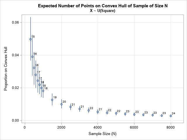
The graph shows the expected proportion of points on the convex hull for samples of size N. The expected number of points (rounded to the nearest integer) is shown adjacent to each marker. For example, you should expect a sample of size N=2000 to have about 1% of its points (k=20) on the convex hull. As the sample size grows larger, the proportion decreases. For N=8000, the expected proportion is only about 0.3%, or 23.5 points on the convex hull.

Simulate samples from the bivariate normal distribution

The previous graph shows the results for points drawn uniformly at random from the unit square. If you change the distribution of the points, you will change the graph. For example, a bivariate normal distribution has most of its points deep inside the convex hull and very few points near the convex hull. Intuitively, you would expect the ratio k / N to be smaller for bivariate normal data, as compared to uniformly distributed data.

You can analyze bivariate normal data by changing only one line of the previous program. Simply change the statement Distrib = "Uniform" to Distrib = "Normal". With that modification, the program creates the following graph:

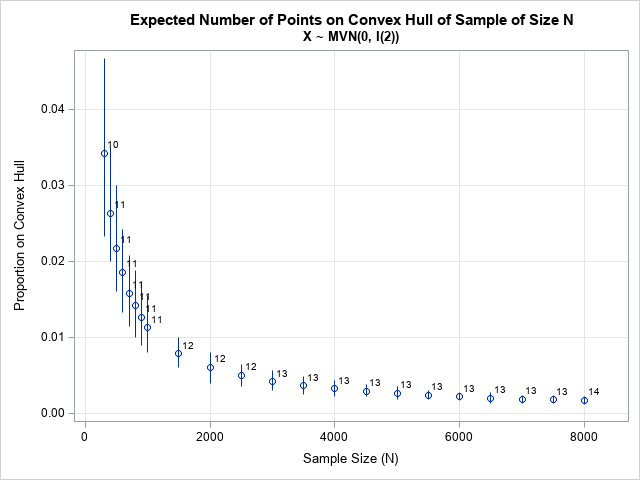
For bivariate normal data, the graph shows that the expected proportion of points on the convex hull is much less than for data drawn from the uniform distribution on the square. For a sample of size N=2000, you should expect about 0.6% of its points (k=12) on the convex hull. For N=8000, the expected proportion is only about 0.2%, or 13.7 points on the convex hull.

Simulate samples from the uniform distribution on the disk

Let's examine one last distribution: the uniform distribution on the unit disk. I have previously shown how to generate random uniform points from the disk, or, in fact, from any d-dimensional ball. The following program defines the RandBall subroutine, which generates random samples from the unit disk. The function is used instead of the RANDGEN subroutine:

/* 4. random uniform in disk: X ~ U(Disk)
   https://blogs.sas.com/content/iml/2016/03/30/generate-uniform-2d-ball.html */
start RandBall(X, radius=1);
   N = nrow(X); d = ncol(X);
   call randgen(X, "Normal");       /* X ~ MVN(0, I(d)) */
   u = randfun(N, "Uniform");       /* U ~ U(0,1)       */
   r = radius * u##(1/d);           /* r proportional to d_th root of U */
   X = r # X / sqrt(X[,##]);        /* X[,##] is sum of squares for each row */
finish;
 
NRep = 250;  /* Monte Carlo simulation: use 250 samples of size N */
N = do(300, 900, 100) || do(1000, 8000, 500);  /* sample sizes */
k = j(NRep, ncol(N), 0);         /* store the number of points on CH */
do i = 1 to ncol(N);
   X = j(N[i], 2, 0);            /* allocate matrix for sample */
   do j = 1 to NRep;
      call RandBall(X);          /* random sample */
      Indices = cvexhull(X);
      k[j,i] = sum(Indices>0);   /* the positive indices are on CH */
   end;
end;
 
p = k / N;                       /* proportion of points on the CH */
mean = mean(p);                  /* expected proportion */
call qntl(CI, p, {0.025, 0.975});  /* 95% confidence interval */
 
title "Expected Number of Points on Convex Hull of Sample of Size N";
title2 "X ~ U(Disk)";
run HiLow(N, mean, CI[1,], CI[2,]);

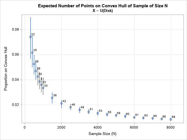
For this distribution, a greater proportion of points are on the convex hull, as compared to the other examples. For a sample of size N=2000, you should expect about 2% of its points (k=42) on the convex hull. For N=8000, the expected proportion is about 0.8%, or 67.7 points on the convex hull.

According Har-Peled (2011), the asymptotic formula for the expected number of points on the convex hull of the unit disk is O(n^1/3).

Linear transformations of convex hulls

Although I ran simulations for the uniform distribution on a square and on a disk, the same results hold for arbitrary rectangles and ellipses. It is not hard to show that if X is a set of points and C(X) is the convex hull, then for any affine transformation T: R² → R², the set T(C(X)) is the convex hull of T(X). Thus, for invertible transformations, the number of points on the convex hull is invariant under affine transformations.

In the same way, the simulation for bivariate normal data (which used uncorrelated variates) remains valid for correlated normal data. This is because the Cholesky transformation maps correlated variates to uncorrelated variates.

Summary

This article uses simulation to understand how the size of a convex hull relates to the size of the underlying sample, drawn randomly from a 2-D distribution. Convex hulls are preserved under linear transformations, so you can simulate from a standardized distribution. This article presents results for three distributions: the uniform distribution on a rectangle, the bivariate normal distribution, and the uniform distribution on an ellipse.