This article uses an example to introduce to genetic algorithms (GAs) for optimization. It discusses two operators (mutation and crossover) that are important in implementing a genetic algorithm. It discusses choices that you must make when you implement these operations.

Some programmers love using genetic algorithms. Genetic algorithms are heuristic methods that can be used to solve problems that are difficult to solve by using standard discrete or calculus-based optimization methods. A genetic algorithm tries to mimic natural selection and evolution by starting with a population of random candidates. Candidates are evaluated for "fitness" by plugging them into the objective function. The better candidates are combined to create a new set of candidates. Some of the new candidates experience mutations. Eventually, over many generations, a GA can produce candidates that approximately solve the optimization problem. Randomness plays an important role. Re-running a GA with a different random number seed might produce a different solution.

Critics of genetic algorithms note two weaknesses of the method. First, you are not guaranteed to get the optimal solution. However, in practice, GAs often find an acceptable solution that is good enough to be used. The second complaint is that the user must make many heuristic choices about how to implement the GA. Critics correctly note that implementing a genetic algorithm is as much an art as it is a science. You must choose values for hyperparameters and define operators that are often based on a "feeling" that these choices might result in an acceptable solution.

This article discusses two fundamental parts of a genetic algorithm: the crossover and the mutation operators. The operations are discussed by using the binary knapsack problem as an example. In the knapsack problem, a knapsack can hold W kilograms. There are N objects, each with a different value and weight. You want to maximize the value of the objects you put into the knapsack without exceeding the weight. A solution to the knapsack problem is a 0/1 binary vector b. If b[i]=1, the i_th object is in the knapsack; if b[i]=0, it is not.

A brief overview of genetic algorithms

The SAS/IML User's Guide provides an overview of genetic algorithms. The main steps in a genetic algorithm are as follows:

• Encoding: Each potential solution is represented as a chromosome, which is a vector of values. The values can be binary, integer-valued, or real-valued. (The values are sometimes called genes.) For the knapsack problem, each chromosome is an N-dimensional vector of binary values.
• Fitness: Choose a function to assess the fitness of each candidate chromosome. This is usually the objective function for unconstrained problems, or a penalized objective function for problems that have constraints. The fitness of a candidate determines the probability that it will contribute its genes to the next generation of candidates.
• Selection: Choose which candidates become parents to the next generation of candidates.
• Crossover (Reproduction): Choose how to produce children from parents.
• Mutation: Choose how to randomly mutate some children to introduce additional diversity.

This article discusses the crossover and the mutation operators.

The mutation operator

The mutation operator is the easiest operation to understand. In each generation, some candidates are randomly perturbed. By chance, some of the mutations might be beneficial and make the candidate more fit. Others are detrimental and make the candidate less fit.

For a binary chromosome, a mutation consists of changing the parity of some proportion of the elements. The simplest mutation operation is to always change k random elements for some hyperparameter k < N. A more realistic mutation operation is to choose the number of sites randomly according to a binomial probability distribution with hyperparameter p_mut. Then k is a random variable that differs for each mutation operation.

The following SAS/IML program chooses p_mut=0.2 and defines a subroutine that mutates a binary vector, b. In this example, there are N=17 items that you can put into the knapsack. The subroutine first uses the Binom(p_mut, N) probability distribution to obtain a random number of sites, k, to mutate. (But if the distribution returns 0, set k=1.) The SAMPLE function then draws k random positions (without replacement), and the values in those positions are changed.

proc iml;
call randseed(12345);
N = 17;                      /* size of binary vector */
ProbMut= 0.2;                /* mutation in 20% of sites */
 
/* Mutation operator for a binary vector, b. 
   The number of mutation sites k ~ Binom(ProbMut, N), but not less than 1. 
   Randomly sample (without replacement) k sites. 
   If an item is not in knapsack, put it in; if an item is in the sack, take it out. */
start Mutate(b) global(ProbMut);
   N = nrow(b);
   k = max(1, randfun(1, "Binomial", ProbMut, N)); /* how many sites? */
   j = sample(1:N, k, "NoReplace");                /* choose random elements */
   b[j] = ^b[j];                                   /* mutate these sites */
finish;
 
Items = 5:12;                  /* choose items 5-12 */
b = j(N,1,0);  b[Items] = 1;
bOrig = b;
run Mutate(b);
print (bOrig`)[L="Original b" c=(1:N)]
      (b`)[L="Randomly Mutated b" c=(1:N)];

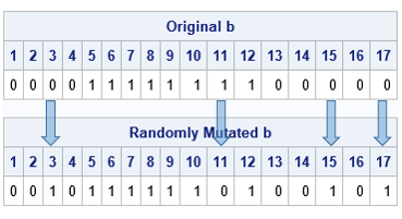
In this example, the original chromosome has a 1 in locations 5:12. The binomial distribution randomly decides to mutate k=4 sites. The SAMPLE function randomly chooses the locations 3, 11, 15, and 17. The parity of those sites is changed. This is seen in the output, which shows that the parity of these four sites differs between the original and the mutated b vector.

Notice that you must choose HOW the mutation operator works, and you must choose a hyperparameter that determines how many sites get mutated. The best choices depend on the problem you are trying to solve. Typically, you should choose a small value for the probability p_mut so that only a few sites are mutated.

In the SAS/IML language, there are several built-in mutation operations that you can use. They are discussed in the documentation for the GASETMUT subroutine.

The crossover operator

The crossover operator is analogous to the creation of offspring through sexual reproduction. You, as the programmer, must decide how the parent chromosomes, p1 and p2, will combine to create two children, c1 and c2. There are many choices you can make. Some reasonable choices include:

• Randomly choose a location s, 1 ≤ s ≤ N. You then split the parent chromosomes at that location and exchange and combine the left and right portions of the parents' chromosomes. One child chromosome is c1 = p1[1:s] // p2[s+1:N] and the other is c2 = p2[1:s] // p1[s+1:N]. Note that each child gets some values ("genes") from each parent.
• Randomly choose a location s, 1 ≤ s ≤ N. Divide the first chromosome into subvectors of length s and N-s. Divide the second chromosome into subvectors of length N-s and s. Exchange the subvectors of the same length to form the child chromosomes.
• Randomly choose k locations. Exchange the locations between parents to form the child chromosomes.

The following SAS/IML function implements the third crossover method. The method uses a hyperparameter, p_cross, which is the probability that each location in the chromosome is selected. On average, about Np_cross locations will be selected. In the following program, p_cross = 0.3, so we expect 17(0.3)=5.1 values to be exchanged between the parent chromosomes to form the children:

start uniform_cross(child1, child2, parent1, parent2) global(ProbCross);
   b = j(nrow(parent1), 1);
   call randgen(b, "Bernoulli", ProbCross); /* 0/1 vector */
   idx = loc(b=1);                    /* locations to cross */
 
   child1 = parent1;                  /* initialize children */
   child2 = parent2;
   if ncol(idx)>0 then do;            /* exchange values */
      child1[idx] = parent2[idx];     /* child1 gets some from parent2 */
      child2[idx] = parent1[idx];     /* child2 gets some from parent1 */
   end;
finish;
 
ProbCross = 0.3;                               /* crossover 25% of sites */
Items = 5:12;   p1 = j(N,1,0);  p1[Items] = 1; /* choose items 5-12 */
Items = 10:15;  p2 = j(N,1,0);  p2[Items] = 1; /* choose items 10-15 */
run uniform_cross(c1, c2, p1, p2);
print (p1`)[L="Parent1" c=(1:N)], (p2`)[L="Parent2" c=(1:N)],
      (c1`)[L="Child1" c=(1:N)], (c2`)[L="Child2" c=(1:N)];

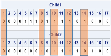
I augmented the output to show how the child chromosomes are created from their parents. For this run, the selected locations are 1, 8, 10, 12, and 14. The first child gets all values from the first parent except for the values in these five positions, which are from the second parent. The second child is formed similarly.

When the parent chromosomes resemble each other, the children will resemble the parents. However, if the parent chromosomes are very different, the children might not look like either parent.

Notice that you must choose HOW the crossover operator works, and you must choose a hyperparameter that determines how to split the parent chromosomes. In more sophisticated crossover operations, there might be additional hyperparameters, such as the probability that a subchromosome from a parent gets reversed in the child. There are many heuristic choices to make, and the best choice is not knowable.

In the SAS/IML language, there are many built-in crossover operations that you can use. They are discussed in the documentation for the GASETCRO subroutine.

Summary

Genetic algorithms can solve optimization problems that are intractable for traditional mathematical optimization algorithms. But the power comes at a cost. The user must make many heuristic choices about how the GA should work. The user must choose hyperparameters that control the probability that certain events happen during mutation and crossover operations. The algorithm uses random numbers to generate new potential solutions from previous candidates. This article used the SAS/IML language to discuss some of the choices that are required to implement these operations.

A subsequent article discusses how to implement a genetic algorithm in SAS.