A genetic algorithm (GA) is a heuristic optimization technique. The method tries to mimic natural selection and evolution by starting with a population of random candidates. Candidates are evaluated for "fitness" by plugging them into the objective function. The characteristics of the better candidates are combined to create a new set of candidates. Some of the new candidates experience mutations. Eventually, over many generations, a GA can produce candidates that approximately solve the optimization problem. This article uses SAS/IML to implement a genetic algorithm in SAS.

A previous article discusses the mutation and crossover operators, which are important in implementing a genetic algorithm. In previous articles, the solution vectors were represented by column vectors. In the GA routines, candidates are row vectors. The population is a matrix, where each row represents an individual.

The main steps in a genetic algorithm

The SAS/IML User's Guide provides an overview of genetic algorithms. The five main steps follow:

• Encoding: Each potential solution is represented as a chromosome, which is a vector of values. For the knapsack problem, each chromosome is an N-dimensional vector of binary values.
• Fitness: Choose a function to assess the fitness of each candidate chromosome. This is usually the objective function for unconstrained problems, or a penalized objective function for problems that have constraints. The fitness of a candidate determines the probability that it will contribute its genes to the next generation of candidates.
• Selection: Choose which candidates become parents to the next generation of candidates.
• Crossover (Reproduction): Choose how to produce children from parents.
• Mutation: Choose how to randomly mutate some children to introduce additional diversity.

Encoding a solution vector

Each potential solution is represented as an N-dimensional vector of values. For the knapsack problem, you can choose a binary vector. In SAS/IML, you use the GASETUP function to define the encoding for a problem. The SAS/IML language supports four different encodings. The knapsack problem can be encoded by using an integer vector, as follows:

/* Individuals are ROW vectors. Population is a matrix of stacked rows. */
proc iml;
call randseed(12345);
/* Solve the knapsack problem: max Value*b  subject to Weight*b <= WtLimit */
/* Item:  1 2 3 4 5   6   7   8   9  10  11  12  13  14  15  16  17 */
Weight = {2 3 4 4 1.5 1.5 1   1   1   1   1   1   1   1   1   1   1}`;
Value  = {6 6 6 5 3.1 3.0 1.5 1.3 1.2 1.1 1.0 1.1 1.0 1.0 0.9 0.8 0.6}`;
WtLimit = 9;                                 /* weight limit */
N = nrow(Weight);
 
/* set up an encoding for the GA */
id = gaSetup(2,                 /* 2-> integer vector encoding */
             nrow(weight),      /* size of vector */
             123);              /* internal seed for GA */

The GASETUP function returns an identifier for the problem. This identifier must be used as the first argument to subsequent calls to GA routines. It is possible to have a program that runs several GAs, each with its own identifier. The GASETUP call specifies that candidate vectors are integer vectors. Later in the program, you can tell the GA that they are binary vectors.

Fitness, mutation, and reproduction

In previous articles, I discussed fitness, mutation, and crossover functions:

• You can use a penalized objective function to evaluate the fitness of a candidate solution.. In the SAS/IML language, use the GASETOBJ subroutine to register the objective function and to specify whether the GA should minimize or maximize the function.
• You can define a mutation subroutine to control how candidates get mutated. You can register the mutation module by using the GASETMUT subroutine. When you call the GASETMUT subroutine, you also need to specify the probability that a candidate will be mutated.
• You can define a crossover subroutine to control how two parents produce two children. You can register the crossover module by using the GASETCRO subroutine. When you call the GASETCRO subroutine, you also need to specify the probability that a fit candidate in the current generation is chosen to reproduce and thus contribute its characteristics to the next generation.

The following SAS/IML statements define the fitness module (ObjFun), the mutation module (Mutate), and the crossover module (Cross) and register these modules with the GA system.

/* just a few of the many hyperparameters */
lambda = 100;       /* factor to penalize exceeding the weight limit */
ProbMut= 0.2;       /* probability that the i_th site is mutated */
ProbCross = 0.3;    /* children based on 30%-70% split of parents */
 
/* b is a binary column vector */
start ObjFun( b ) global(Weight, Value, WtLimit, lambda);
   wsum = b * Weight;
   val  = b * Value;
   if wsum > WtLimit then                      /* penalize if weight limit exceeded */
      val = val - lambda*(wsum - WtLimit)##2;  /* subtract b/c we want to maximize value */
   return(val);
finish;
 
/* Mutation operator for a binary vector, b. */
start Mutate(b) global(ProbMut);
   N = ncol(b);
   k = max(1, randfun(1, "Binomial", ProbMut, N)); /* how many sites? */
   j = sample(1:N, k, "NoReplace");                /* choose random elements */
   b[j] = ^b[j];                                   /* mutate these sites */
finish;
 
/* Crossover operator for a a pair of parents. */
start Cross(child1, child2, parent1, parent2) global(ProbCross);
   b = j(ncol(parent1), 1);
   call randgen(b, "Bernoulli", ProbCross); /* 0/1 vector */
   idx = loc(b=1);                          /* locations to cross */
   child1 = parent1;
   child2 = parent2;
   if ncol(idx)>0 then do;                  /* exchange values */
      child1[idx] = parent2[idx];
      child2[idx] = parent1[idx];
   end;
finish;
 
/* register these modules so the GA can call them as needed */
call gaSetObj(id, 1, "ObjFun"); /* 1->maximize objective module */
call gaSetCro(id,
              1.0,              /* hyperparameter: crossover probability */
              0, "Cross");      /* user-defined crossover module */
call gaSetMut(id,
              0.20,             /* hyperparameter: mutation probability */
              0, "Mutate");     /* user-defined mutation module */

Fitness and selection

A genetic algorithm pits candidates against each other according to Darwin's observation that individuals who are fit are more likely to pass on their characteristics to the next generation.

A genetic algorithm evolves the population across many generations. The individuals who are more fit are likely to "reproduce" and send their progeny to the next round. To preserve the characteristics of the very best individuals (called elites), some individuals are "cloned" and passed unchanged to the next generations. After many rounds, the population is fitter, on average, and the elite individuals are the best solutions to the objective function.

In SAS/IML, you can use the GASETSEL subroutine to specify the rules for selecting elite individuals and for are selecting which individuals are eligible to reproduce. The following call specifies that 3 elite individuals are "cloned" for the next generation. For the remaining individuals, pairs are selected at random. With 95% probability, the more fit individual is selected to reproduce:

call gaSetSel(id,
              3,                /* hyperparameter: carry k elites directly to next generation */
              1,                /* dual tournament */
              0.95);            /* best-player-wins probability */

At this point, the GA problem is fully defined.

Initial population and evolution

You can use the GAINIT subroutine to generate the initial population. Typically, the initial population is generated randomly. If there are bounds constraints on the solution vector, you can specify them. For example, the following call generates a very small population of 10 random individuals. The chromosomes are constrained to be binary by specifying a lower bound of 0 and an upper bound of 1 for each element of the integer vector.

/* example of very small population; only 10 candidates */
call gaInit(id,  10,            /* initial population size */
            j(1,  nrow(weight), 0) //   /* lower and upper bounds of binary vector */
            j(1,  nrow(weight), 1) );

You can evolve the population by calling the GAREGEN subroutine. The GAREGEN call selects individuals to reproduce according to the tournament rules. The selected individuals become parents. Pairs of parents produce children according to the crossover operation. Some children are mutated according to the mutation operator. The children become the next generation and replace the parents as the "current" population.

At any time, you can use the GAGETMEM subroutine to obtain the members of the current population. You can use the GAGETVAL subroutine to obtain the fitness scores of the current population. Let's manually call the GAREGEN subroutine a few times and use the GAGETVAL subroutine after each call to see how the population evolves:

call gaGetVal(f0, id);     /* initial generation is random */ 
call gaRegen(id);          /* create the next generation via selection, crossover, and mutation */
call gaGetVal(f1, id);     /* evaluate fitness */
call gaRegen(id);          /* continue for additional generations ...*/
call gaGetVal(f2, id);
 
/* print fitness for each generation and top candidates so far */
print f0[L="Initial Fitness"] f1[L="1st Gen Fitness"] f2[L="2nd Gen Fitness"];
call gaGetMem(best, val, id, 1:3);
print best[f=1.0 L="Best Members"], val[L="Best Values"];

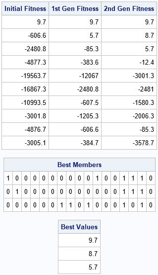
The output shows how the population evolves for three generations. Initially, only one member of the population satisfies the weight constraints of the knapsack problem. The feasible solution has a positive fitness score (9.7); the infeasible solutions are negative for this problem. After the selection, crossover, and mutation operations, the next generation has two feasible solutions (9.7 and 8.1). After another round, the population has six feasible solutions and the score for the best solution has increased to 11.7. The population is becoming more fit, on average.

After the second call to GAREGEN, the GAGETMEM call gets the candidates in positions 1:3. Recall that you specified three "elite" members in the GASETSEL call. The elite members are therefore placed at the top of the population. (The remaining individuals are not sorted according to fitness.) The chromosomes for the elite members are shown. In this encoding, each chromosome is a 0/1 binary vector that determines which objects are placed in the knapsack and which are left out.

Evolution towards a solution

The previous section purposely used a small population of 10 individuals. Such a small population lacks genetic diversity and might not converge to an optimal solution (or at least not quickly). A more reasonable population contains 100 or more individuals. You can use the GAINIT call a second time to reinitialize the initial population. Now that you have experience with the GAREGEN and GAGETVAL calls, you can use those calls in a DO loop to iterate over many generations. The following statements iterate the initial population through 15 generations. For each generation, the program records the best fitness score (f[1]) and the median fitness score.

/* for genetic diversity, better to have a larger population */
call gaInit(id,  100,                   /* initial population size */
            j(1,  nrow(weight), 0) //   /* lower and upper bounds of binary vector */
            j(1,  nrow(weight), 1) );   
/* record the best and median scores for each generation */
niter = 15;
summary = j(niter,3);
summary[,1] = t(1:niter);   /* (Iteration, Best Value, Median Value) */
do i = 1 to niter;
   call gaRegen(id);
   call gaGetVal(f, id);
   summary[i,2] = f[1];   summary[i,3] = median(f);
end;
print summary[c = {"Iteration" "Best Value" "Median Value"}];

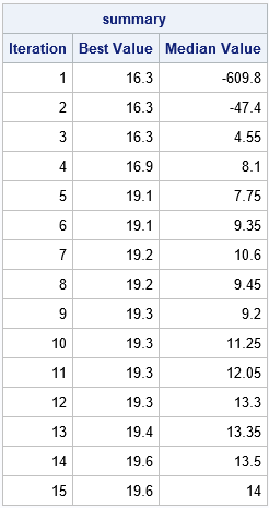
The output shows that the fitness of the best candidate is monotonic. It increases from an initial value of 16.3 to the final value of 19.6, which is the optimal value. Similarly, the median value tends to increase. Because of random mutation and the crossover operations, statistics such as the median or mean are usually not monotonic. Nevertheless, the fitness of later generations tends to be better than for earlier generations.

You can examine the chromosomes of the elite candidates in the final generation by using the GAGETMEM subroutine:

/* print the top candidates */
call gaGetMem(best, f, id, 1:3);
print best[f=1.0 L="Best Member"], f[L="Final Best Value"];

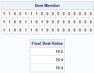
The output confirms that the best candidate is the same binary vector as was found by using a constrained linear program in a previous article.

The GA algorithm maintains an internal state, which enables you to continue iterating if the current generation is not satisfactory. In this case, the problem is solved, so you can use the GAEND subroutine to release the internal memory and resources that are associated with this GA. After you call GAEND, the identifier becomes invalid.

call gaEnd(id);   /* free the memory and internal resources for this GA */

The advantages and disadvantage of genetic algorithms

As with any tool, it is important to recognize that a GA has strengths and weaknesses. Strengths include:

• A GA is amazingly flexible. It can be used to solve a wide variety of optimization problems.
• A GA can provide useful suboptimal solutions. The elite members of a population might be "good enough," even if they are not optimal.

Weaknesses include:

• A GA is dependent on random operations. If you change the random number seed, you might obtain a completely different solution or no solution at all.
• A GA can take a long time to produce an optimal solution. It does not tell you whether a candidate is optimal, only that it is the "most fit" so far.
• A GA requires many heuristic choices. It is not always clear how to implement the mutation and crossover operators or how to implement the tournament that selects individuals to be parents.

Summary

In summary, this article shows how to use low-level routines in SAS/IML software to implement a genetic algorithm. Genetic algorithms can solve optimization problems that are intractable for traditional mathematical optimization algorithms. Like all tools, a GA has strengths and weaknesses. By gaining experience with GAs, you can build intuition about when and how to apply this powerful method.

For other ways to use genetic algorithms in SAS, see the GA procedure in SAS/OR software and the black-box solver in PROC OPTMODEL.