Many optimization problems in statistics and machine learning involve continuous parameters. For example, maximum likelihood estimation involves optimizing a log-likelihood function over a continuous domain, possibly with constraints. Recently, however, I had to solve an optimization problem for which the solution vector was a 0/1 binary variable. To solve the problem, I used the MILPSOLVE subroutine in SAS/IML. The MILPSOLVE subroutine can solve general mixed integer linear programming (MILP) problems. Solving for a binary solution vector is a simple application of using the MILPSOLVE subroutine.

The knapsack problem

To demonstrate how to solve for a binary solution vector, let's consider a famous type of optimization problem called the knapsack problem. Suppose that a knapsack can hold W kilograms. There are N objects, each with a different value and weight. You want to maximize the value of the objects you put into the knapsack without exceeding the weight.

A solution to the knapsack problem is a 0/1 binary vector b. If b[i]=1, you put the i_th object into the knapsack; if b[i]=0, you do not. If w is a vector of weights and v is a vector of values, then the knapsack problem seeks to maximize the sum of the values subject to the constraint that the sum of the weights does not exceed W. In symbols, maximize v`*b such that w`*b ≤ W.

Let's create and solve an example that has 17 items. The following SAS/IML statements define a weight vector and a vector of values for the objects. By default, the MILPSOLVE subroutine assumes that the solution vector is binary, so we do not have to specify the type of solution that we are searching for. The only information we must specify is the type of the problem (maximize or minimize) and the "sense" of the constraint (=, ≤, or ≥). The following statements define and solve the knapsack problem for the 17 items:

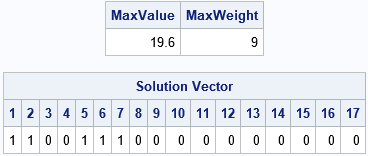
/* The (binary) Knapsack Problem:
   max value*b
   s.t. weight*b <= WtLimit
   b[i] is binary 0/1
*/
proc iml;
/* Item:  1 2 3 4 5   6   7   8   9  10  11  12  13  14  15  16  17 */
weight = {2 3 4 4 1.5 1.5 1   1   1   1   1   1   1   1   1   1   1};
Value  = {6 6 6 5 3.1 3.0 1.5 1.3 1.2 1.1 1.0 1.1 1.0 1.0 0.9 0.8 0.6};
WtLimit = 9;                                 /* weight limit */
 
rowsense = "L";                              /* L = 'less than or equal' */
cntl = -1;                                   /* maximize the objective */
call milpsolve(rc, MaxValue, b, relgap,      /* output args */
               Value, Weight, WtLimit)       /* required input args */
               CNTL=cntl ROWSENSE=rowsense;  /* optional args */
/* Check the weight of the solution. Print the max value and the solution vector */
MaxWeight = Weight*b;
print MaxValue MaxWeight, /* MaxValue  = Value*b */
      (b`)[L="Solution Vector" c=(1:nrow(b))];

The solution is to place items 1, 2, 5, 6, and 7 into the knapsack. The total weight of these items is 9 kg. The value of these items is 19.6, which is the most value that you can put into the knapsack, given the weight constraint.

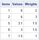
The following statements print the items, values, and weights of the optimal solution:

/* print weights and values for the selected items */
Items = T( loc(b) );            /* select items where b=1 */
Values = Value[Items];          /* values of selected items */
Weights = Weight[Items];        /* weights of selected items */
print Items Values Weights;

You can mentally verify that the weight of these items does not exceed 9 kg.

Summary

The MILPSOLVE subroutine in SAS/IML software can solve mixed integer linear programming problems. The simplest example of these kinds of problems is finding a binary solution vector. Binary solution vectors are often used to indicate whether some quantity is included or omitted. The classical knapsack problem is an example of an optimization problem whose solution vector is binary. This article shows how to solve the knapsack problem by using the MILPSOLVE subroutine in SAS/IML.