Sometimes we can learn as much from our mistakes as we do from our successes. Recently, I needed to solve an optimization problem for which the solution vector was a binary vector subject to a constraint. I was in a hurry. Without thinking much about what I was doing, I decided to eliminate the constraint by introducing a penalty term into the objective function. I then solved the unconstrained penalized optimization problem. A few days later, I thought further about what I had done. I had reformulated a constrained optimization problem as an unconstrained penalized optimization. Was that a wise (or valid!) thing to do? Are there issues that I should have considered before I took reformulated the problem?

The knapsack problem

I recently wrote about how to solve a famous optimization problem called the knapsack problem. In the knapsack problem, you assume that a knapsack can hold W kilograms. There are N objects whose values and weights are represented by elements of the vectors v and w, respectively. The goal is to maximize the value of the objects you put into the knapsack without exceeding a weight constraint, W.

As shown in my previous article, the knapsack problem can be solved by using integer linear programming to find a binary (0/1) solution vector that maximizes v`*b subject to the constraint w`*b ≤ W.

The problem I needed to solve was similar to the knapsack problem, so let's examine what happens if you reformulate the knapsack problem to eliminate the constraint on the weights. The idea is to introduce a penalty for any set of weights that exceed the limit. For example, if a candidate set of items have weight W_c > W, then you could subtract a positive quantity such as λ*(W_c - W)². If the penalty parameter λ > 0 is large enough, then subtracting the penalty term will not affect the optimal solution, which we are trying to maximize. (If you are minimizing an objective function, then ADD a positive penalty term.) Notice that the penalty term destroys the linearity of the objective function.

A penalized knapsack formulation

The following SAS/IML program demonstrates how to use an IF-THEN statement to include a penalty term in the objective function for the knapsack problem:

proc iml;
/* Solve the knapsack problem: max Value*b  subject to Weight*b <= WtLimit */
/* Item:  1 2 3 4 5   6   7   8   9  10  11  12  13  14  15  16  17 */
Weight = {2 3 4 4 1.5 1.5 1   1   1   1   1   1   1   1   1   1   1};
Value  = {6 6 6 5 3.1 3.0 1.5 1.3 1.2 1.1 1.0 1.1 1.0 1.0 0.9 0.8 0.6};
WtLimit = 9;                                 /* weight limit */
N = ncol(Weight);
lambda = 10;       /* factor to penalize exceeding the weight limit */
 
/* b is a binary column vector */
start ObjFun( b ) global(Weight, Value, WtLimit, lambda);
   wsum = Weight * b;
   val  = Value * b;
   if wsum > WtLimit then                      /* penalize if weight limit exceeded */
      val = val - lambda*(wsum - WtLimit)##2;  /* subtract b/c we want to maximize value */
   return(val);
finish;
 
/* call the objective function on some possible solution vectors */
Items = 5:12;                  /* choose items 5-12 */
b = j(N,1,0);  b[Items] = 1;
ValPen = ObjFun(b);            /* values penalized if too much weight */
ValUnPen = Value*b;            /* raw values, ignoring the weights */
Wt = Weight*b;                 /* total weight of items */
print (ValPen||ValUnpen||Wt)[L="Items 5:12" 
    c={"Penalized Value" "Unpenalized Value" "Weight"}];
 
Items = 5:13;                  /* choose items 5-13 */
b = j(N,1,0);  b[Items] = 1;
ValPen = ObjFun(b);            /* values penalized if too much weight */
ValUnPen = Value*b;            /* raw values, ignoring the weights */
Wt = Weight*b;                 /* total weight of items */
print (ValPen||ValUnpen||Wt)[L="Items 5:13" 
    c={"Penalized Value" "Unpenalized Value" "Weight"}];

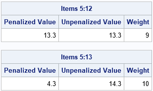
In the first example (Items 5:12), the weight of the items does not exceed the weight limit. Therefore, the objective function returns the actual value of the items. In the second example (Items 5:13), the weight of the items is 10, which exceeds the weight limit. Therefore, the objective function applies the penalty term. Instead of returning 14.3 as the value of the items, the function returns 4.3, which is 10 less because the penalty term evaluates to -10*1² for this example.

You can visualize how the penalty works by generating many random binary vectors. The following statements generate 1,000 random binary vectors where the probability of generating a 1 is 0.3. For each random vector, the program calls the penalized objective function to obtain a (penalized) value of the items. A scatter plot displays the penalized value versus the weight of the items.

/* generate 1,000 random binary vectors as columns of b */
call randseed(1234);
NumSim = 1000;
Val = j(NumSim, 1, .);
b = randfun(N||NumSim, "Bernoulli", 0.3);
do i = 1 to NumSim;
   Val[i] = ObjFun(b[,i]);
end;
Wt  = Weight * b;
 
title  "Value of 1,000 Random Knapsacks";
title2 "b ~ Bern(0.3); lambda=10";
call scatter(Wt, Val) grid={x y} label={"Weight"}
             other = "refline 9 / axis=x; yaxis min=-20 label='Value';";

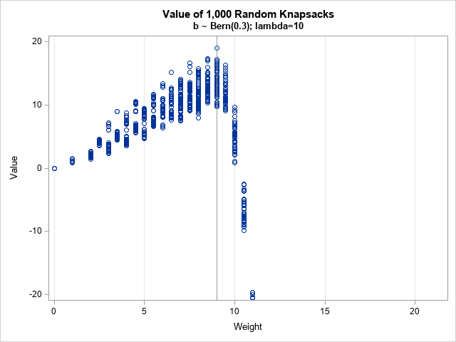
For each random binary vector, the ObjFun function returns the penalized value. The graph shows that, on average, the penalized value peaks when the weight is 9 kg, which is the maximum weight the knapsack can hold. If the collective weight of the items exceeds 10, the "value" is actually NEGATIVE for this example! Although the graph shows only 1,000 random choices for the b vector, it is representative of the behavior for the full 2¹⁷ = 131,072 possible values of b.

Notice that the largest value achieved by these random binary vectors occurs when the sum of weights is 9, which is the constraint. However, if you use a smaller value for the penalty parameter (such as λ=1) and rerun the simulation, the largest values of the penalized objective function can occur for weights that exceed the constraint. Try it!

The graph provides evidence that you can maximize the unconstrained penalized objective function and find the same optimal value, provided that the coefficient of the penalty term is large enough.

Choosing the penalty term: A little bit of math

What does "large enough" mean? In the example, I used λ=10, but is 10 large enough? Can you find a value for λ that guarantees that the solution of the penalized problem satisfies the constraint?

Let's examine how to choose the penalty parameter, λ. Suppose your goal is to maximize a function f(x) subject to the general constraint that g(x) ≤ 0 for some function g. You can define a penalty function, p(x), which has the property p(x) = 0 whenever g(x) ≤ 0, and p(x) > 0 whenever g(x) > 0. A common choice is a quadratic penalty such as p(x) = |max(0, g(x))|². You then maximize the penalized objective function q(x;λ) = f(x) - λp(x) for a large value of the penalty parameter, λ.

Suppose that b^* is an optimal solution and V^* is the optimal value. For an arbitrary binary vector, b, we want to know whether v * b can be greater than V^* if w * b > W. Let V^* + ΔV be the value and W + ΔW be the weight of the items that are selected by b. Then the penalized objective function is
V^* + ΔV - λ(ΔW)²
and we want to choose λ so large that
V^* + ΔV - λ(ΔW)² ≤ V^*
Solving for λ gives
λ ≥ ΔV / (ΔW)²

You can examine the data to find a lower bound for λ. You want the numerator to be as large as possible and the denominator to be as small as possible. The largest value for the numerator is the total value of the items, sum(v). The smallest value for the denominator is the minimum difference between the weights of items, which is 0.5 for this example. Therefore, for this example, λ ≥ 4*sum(v) will ensure that the solution of the unconstrained penalized objective function is also a solution for the constrained problem. This bound is not tight; you can choose a smaller value with a little more effort.

Conclusions

Even if something is possible, it is not necessarily a good idea. Solving a linear problem with linear constraints can be done very efficiently. If you introduce a penalty term, the objective function is no longer linear, and solving the problem might require more computational resources. Now that I think about it, it was a mistake to reformulate my problem.

In summary, I should have been more careful when I reformulated a constrained optimization problem as an unconstrained penalized optimization. The optimal solution to the penalized problem might or might not be an optimal solution to the original problem. By looking carefully at the mathematics of this problem, I gained a better understanding of the relationship between constrained optimization and unconstrained penalized optimization.