In general, it is hard to simulate multivariate data that has a specified correlation structure. Copulas make that task easier for continuous distributions. A previous article presented the geometry behind a copula and explained copulas in an intuitive way. Although I strongly believe that statistical practitioners should be familiar with statistical theory, you do not need to be an expert in copulas to use them to simulate multivariate correlated data. In SAS, the COPULA procedure in SAS/ETS software provides a syntax for simulating data from copulas. This article shows how to use PROC COPULA to simulate data that has a specified rank correlation structure. (Similar syntax applies to the CCOPULA procedure in SAS Econometrics, which can perform simulations in parallel in SAS Viya.)

Example data

Let's choose some example data to use for the simulation study. Suppose you want to simulate data that have marginal distributions and correlations that are similar to the joint distribution of the MPG_City, Weight, and EngineSize variables in the Sashelp.Cars data set. For ease of discussion, I rename these variables X1, X2, and X3 in this article. The following call to PROC CORR visualizes the univariate and bivariate distributions for these data:

/* for ease of discussion, rename vars to X1, X2, X3 */
data Have;
set Sashelp.Cars(keep= MPG_City Weight EngineSize);
label MPG_City= Weight= EngineSize=;
rename MPG_City=X1 Weight=X2 EngineSize=X3;
run;
 
/* graph original (renamed) data */
ods graphics / width=500px height=500px;
proc corr data=Have Spearman noprob plots=matrix(hist);
   var X1 X2 X3;
   ods select SpearmanCorr MatrixPlot;
run;

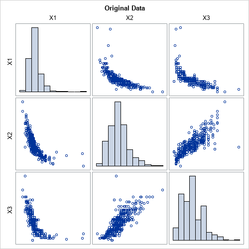
The graph shows the marginal and bivariate distributions for these data. The goal of this article is to use PROC COPULA to simulate a random sample that looks similar to these data. The output from PROC CORR includes a table of Spearman correlations (not shown), which are Corr(X1,X2)=-0.865, Corr(X1,X3)=-0.862, and Corr(X2,X3)=0.835.

Using PROC COPULA to simulate data

As explained in my previous article about copulas, the process of simulating data involves several conceptual steps. For each step, PROC COPULA provides a statement or option that performs the step:

1. The multivariate distribution is defined by specifying a marginal distribution for each variable and a correlation structure for the joint distribution. In my previous article, these were created "out of thin air." However, in practice, you often want to simulate random samples that match the correlation and marginal distributions of real data. In PROC COPULA, you use the DATA= option and the VAR statement to specify real data.
2. Choose a copula family and use the data to estimate the parameters of the copula. I've only discussed the Gaussian copula. For the Gaussian copula, the sample covariance matrix estimates the parameters for the copula, although PROC COPULA uses maximum likelihood estimates instead of the sample covariance. You use the FIT statement to fit the parameters of the copula from the data.
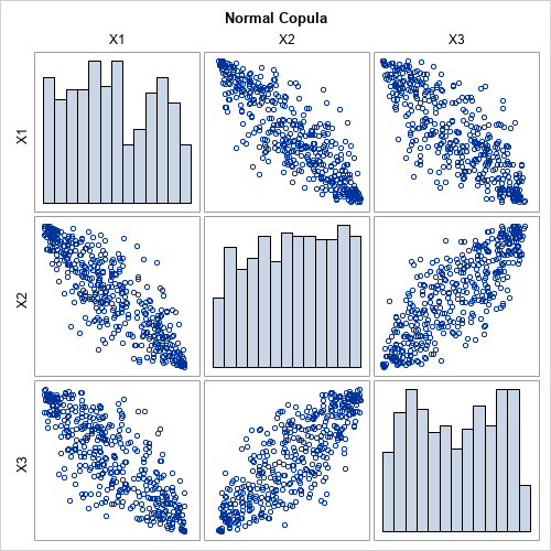
3. Simulate from the copula. For the normal copula, this consists of generating multivariate normal data with the given rank correlations. These simulated data are transformed to uniformity by applying the normal CDF to each component. You use the SIMULATE statement to simulate the data. If you want to see the uniform marginals, you can use the OUTUNIFORM= option to store them to a SAS data set, or you can use the PLOTS=(DATATYPE=UNIFORM) option to display a scatter plot matrix of the uniform marginals.
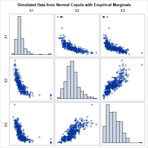
4. Transform the uniform marginals into the specified distributions by applying the inverse CDF transformation for each component. In PROC COPULA, you use the MARGINALS=EMPIRICAL option on the SIMULATE statement to create the marginal distributions by using the empirical CDF of the variables. You can use the OUT= option to write the simulated values to a SAS data set. You can use the PLOTS=(DATATYPE=ORIGINAL) option to display a scatter plot matrix of the simulated data.

The following call to PROC COPULA carries out these steps:

%let N = 428;            /* sample size */
proc copula data=Have;
   var X1 X2 X3;         /* original data vars */
   fit normal;           /* choose normal copula; estimate covariance by MLE */
   simulate / seed=1234 ndraws=&N
              marginals=empirical    /* transform from copula by using empirical CDF of data */
              out=SimData            /* contains the simulated data */
              plots=(datatype=both); /* optional: scatter plots of copula and simulated data */
              /* optional: use OUTUNIFORM= option to store the copula */
   ods select SpearmanCorrelation MatrixPlotSOrig MatrixPlotSUnif;
run;

The primary result of the PROC COPULA call is an output data set called SimData. The data set contains random simulated data. The Spearman correlation of the simulated data is close to the Spearman correlation of the original data. The marginal distributions of the simulated variables are similar to the marginal distributions of the original variables. The following graph shows the distributions of the simulated data. You can compare this graph to the graph of the original data.

When you use PROC COPULA, it is not necessary to visualize the copula, which encapsulates the correlation between the variables. However, if you want to visualize the copula, you can use the PLOTS= option to create a scatter plot matrix of the uniform marginals, as follows:

Use PROC COPULA for Monte Carlo simulations

In Monte Carlo simulations, it is useful to have one SAS data set that contains B simulated samples. You can then use BY-group processing to analyze all simulated samples with a single call to a SAS procedure.

In PROC COPULA, the NDRAWS= option on the SIMULATE statement specifies how many observations to simulate. If your original data contains N observations, you can use NDRAWS=N. To get a total of B simulated samples, you can simulate N*B observations. You can then add an ID variable that identifies which observations belong to each sample, as follows:

/* you can run a Monte Carlo simulation from the simulated data */
%let NumSamples = 1000; /* = B = number of Monte Carlo simulations */
%let NTotal = %eval(&N * &NumSamples);
%put &=NTotal;
 
ods exclude all;
proc copula data=Have;
   var X1 X2 X3;
   fit normal;
   simulate / seed=1234 ndraws=&NTotal marginals=empirical out=SimData;
run;
ods exclude none;
 
/* add ID variable that identifies each set of &N observations */
data MCData;
set SimData;
SampleID = ceil(_N_/&N);  /* 1,1,...,1,2,2,....,2,3,3,... */
run;

You can use your favorite SAS procedure and the BY SAMPLEID statement to analyze each sample in the MCData data set.

Summary

Given a set of continuous variables, a copula enables you to simulate a random sample from a distribution that has the same rank correlation structure and marginal distributions as the specified variables. A previous article discusses the mathematics and the geometry of copulas. In SAS, the COPULA procedure enables you to simulate data from copulas. This article shows how to use PROC COPULA to simulate data. The procedure can create graphs that visualize the simulated data and the copula. The main output is a SAS data set that contains the simulated data.