Compute bivariate ranks

Ranking is a fundamental concept in statistics. Ranks of univariate data are used by statisticians to estimate statistics such as percentiles (quantiles) and empirical distributions. A more advanced use is to compute various rank-based measures of correlation or association between pairs of variables. For example, ranks are used to compute the Spearman rank correlation.

The Spearman correlation uses univariate ranks. That is, the Spearman correlation between variables X and Y is determined by computing the tied ranks for X and Y separately. Other bivariate measures of association use a different type of ranking, which is known as the bivariate rank. In a bivariate ranking, the pairs of (X,Y) values are ranked. A bivariate ranking assigns a rank to the pairs by using the X values, the Y values, and the joint values. This article provides an example of a bivariate ranking scheme, which is used in computing a statistic known as Hoeffding's dependence coefficient.

A formula for a bivariate rank

The SAS/IML language supports the BRANKS function, which computes bivariate (tied) ranks according to the following formula. If the data are pairs of values {(X_i, Y_i) | i=1,2,...,n}, then the bivariate rank of the i_th point is
$Q_i = 3/4 + \sum\nolimits_j u(X_i - X_j) u(Y_i - Y_j)$
where u is a function that counts how many values are less than or equal to a given value. Tied values are counted as 0.5. Specifically, u(t)=1 if t>0, u(t)=1/2 if t=0, and u(t)=0 otherwise.

You can think of the formula as a (scaled) estimate of the bivariate cumulative distribution function (CDF). If you assume that all data values are distinct (no tied values), then the argument to the u function is never 0, and the formula counts how many data points have an X coordinate less than X_i and (simultaneously) a Y coordinate less than Y_i. If the data have tied values in one or both coordinates, then the formula for the rank of P = (X_i, Y_i) says:

Add 1 for every data point that is less than P in both coordinates.
Add 1/2 for every data point that has one coordinate less than P and the other coordinate equal to the corresponding coordinate of P.
Add 1/4 for every data point that is equal to P.

Compute bivariate ranks in SAS

The SAS/IML language supports the BRANKS function, which computes bivariate (tied) ranks according to the formula in the previous section. Let's start with a sample that has nine observations. The ninth observation is a repeat of the eighth observation. The BRANKS function returns a matrix that has three columns:

The first column of the output is the tied ranks (using the MEAN method) of the X coordinate of the data. (You can read a previous article to learn more about univariate tied ranks.)
The second column is the tied ranks of the Y coordinate of the data.
The third column is the bivariate ranks of the (X,Y) values, which is computed by using the formula in the previous section.

/* BIVARIATE RANKS */
proc iml;
w = {10 20, 
     10 21, 
     10 22, 
     11 20, 
     11 21, 
     11 22, 
     12 20, 
     12 22, 
     12 22 };  /* last row is a repeat */
Ranks = branks(w);
print w[c={x y}], Ranks[c={'RankX' 'RankY' 'BRank'}];

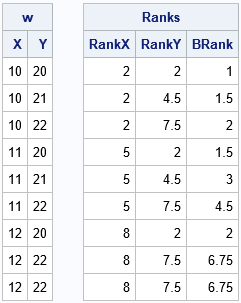
The first two columns are univariate tied ranks of the X and Y coordinates. This third column is the bivariate ranking of the pairs of points. If you think about plotting the points on a scatter plot, points that are in the lower-left corner of the plot have the lowest ranks, and points in the upper-right corner have the higher ranks.

Checking the BRANKS output

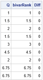
To ensure that the BRANKS function does, in fact, use the formula in the documentation, I wrote the following function, which evaluates the formula "manually." The following statements verify that the formula gives the same values as the third column of the BRANKS function:

/* compute bivariate ranks manually */
start BivarRank(xy);
   x = xy[,1];
   y = xy[,2];
   n = nrow(x);
   Q = j(n, 1, .);
   do i = 1 to n;
      ux = (x[i] > x) + 0.5*(x[i] = x); /* count X values >= x[i] */
      uy = (y[i] > y) + 0.5*(y[i] = y); /* count Y values >= y[i] */
      Q[i] = 0.75 + sum( ux#uy );       /* bivariate rank of (x[i], y[i]) */
   end;
   return Q;
finish;
 
Q = BivarRank(w);
bivarRank = Ranks[,3];
print Q bivarRank (Q-bivarRank)[L="Diff"];

A visualization of bivariate ranks

It's not clear (to me) how this formula assigns ranks to a cloud of points in a scatter plot. We know that the points in the lower-left corner of the graph have low bivariate ranks and that points in the upper-right corner have high bivariate ranks. However, it is not clear what happens in the middle.

Let's generate some data and find out! The following program statements generate 1000 random uniform points in the unit square. The points and the bivariate ranks are written to a SAS data set. PROC SGPLOT displays the points and colors the markers according to the bivariate rank, as follows:

/* compute bivariate ranks for random data */
call randseed(1234);
xy = randfun({1000 2}, "Uniform" );  /* 1000 random uniform points in [0,1]x[0,1] */
bivarRank = branks(xy);              /* third column contains bivariate ranks */
m = bivarRank || xy;
create BivarRanks from m[c={'rx' 'ry' 'brank' 'x' 'y'}];
append from m;
close;
QUIT;
 
/* palette("spectral",9) */
%let colorRamp = CXD53E4F CXF46D43 CXFDAE61 CXFEE08B CXFFFFBF CXE6F598 CXABDDA4 CX66C2A5 CX3288BD;
title "Bivariate Ranks of 1000 Points";
proc sgplot data=BivarRanks aspect=1;
   scatter x=x y=y / colorresponse=brank markerattrs=(symbol=CircleFilled)
   colormodel=(&colorRamp);
run;

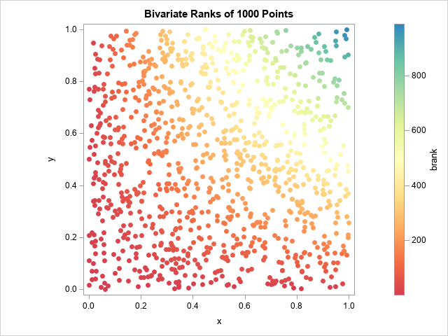
The colors of the markers indicate the bivariate ranks of the observations. The graph indicates that low ranks are assigned to points whose X or Y coordinates are small. High ranks are assigned only when both coordinates are large.

Notice that the ranks are not uniformly distributed among the 1000 points. That is because there are many tied ranks for the lower ranks. For example, about 50% of the points have ranks less than 200. Only 10% have ranks greater than 600.

A connection with bivariate CDF

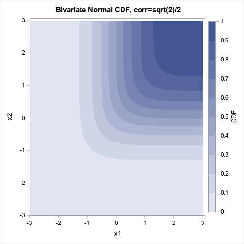
As I indicated earlier, the formula for the bivariate ranks is reminiscent of the definition of a bivariate CDF. In retrospect, I should not have been surprised to see that coloring the observations by their bivariate rank looks a lot like a two-dimensional CDF. For example, the following graph shows the CDF for the bivariate normal distribution:

Summary

This article discusses the concept of a bivariate rank for ordered pairs. In a bivariate rank, both the X and Y coordinate are used to assign a rank. The formula that computes the bivariate rank is not complicated, but I did not initially understand how it assigns ranks to points in a scatter plot. As usual, a visualization helps. The visualization shows that bivariate ranks are conceptually similar to the computation of a two-dimensional CDF.

Blogs