Gaussian random walks and Levy flights

Imagine an animal that is searching for food in a vast environment where food is scarce. If no prey is nearby, the animal's senses (such as smell and sight) are useless. In that case, a reasonable search strategy is a random walk. The animal can choose a random direction, walk/swim/fly in that direction for a while, and hope that it encounters food. If not, it can choose another random direction and try again.

According to a story in Quanta magazine, an optimal search strategy is to use a variant of a random walk that is known as a Lévy flight. This article describes a Lévy flight, simulates it in SAS, and compares it to Gaussian random walk.

Random walks

For the purpose of this article, a 2-D random walk is defined as follows. From the current position,

Choose a random direction by choosing an angle, θ, uniformly in [0, 2π).
Choose a random distance, r.
Move that distance in that direction.

The amount of territory that gets explored during a random walk depends on the distribution of the distances. For example, if you always choose a unit distance, you obtain the "drunkard's walk." If you choose distances from a normal distribution, you obtain a Gaussian walk. In both scenarios, the animal primarily searches near where it has been previously. These random walks that always use short distances are good for finding food in a food-rich environment.

In a food-scarce environment, it is a waste of time and energy to always move a short distance from the previous position. It turns out that a better strategy is to occasionally move a long distance. That puts the animal in a new location, which it can explore by moving small distances again. According to the Quanta article, this behavior has been observed "to greater or lesser extents" in many animals that hunt at sea, including albatross, sharks, turtles, penguins, and tuna (Sims, et al., Nature, 2008).

Levy walks and the Levy distribution

A popular model for this behavior is the Lévy walk, which is often called a Lévy flight because it was first applied to the flight path of an albatross over open water. In a Lévy flight, the distance is a random draw from a heavy-tailed distribution. In this article, I will simulate a Lévy flight by drawing distances from a Lévy distribution, which is a special case of the inverse gamma distribution.

The Lévy distribution Levy(μ, c) has a location parameter (μ) and a shape parameter (c). It is a special case of the inverse gamma distribution, which is represented by IGamma(α, β). If X ~ Levy(μ, c) is a random variable, then X – μ ~ IGamma(1/2, β/2). In this article, μ=0, so a random draw from the Levy(0,c) distribution is a random draw from IGamma(1/2, c/2) distribution. Thus, you can use the SAS program in the previous article to generate a random sample from the Lévy distribution.

The inverse gamma distribution with α=1/2 has very heavy tails. This means that a random variate can be arbitrarily large. When modeling a physical or biological system, there are often practical bounds on the maximum value of a quantity. For example, if you are modeling the flight of an albatross, you know that there is a maximum distance that an albatross can fly in a given time. Thus, researchers often use a truncated Lévy distribution to model the distances that an animal travels in one unit of time. For example, an albatross can fly up to 800 km in one day (!!), so a model of albatross distances should truncate the distances at 800.

Simulate a Gaussian and Levy Walk

You can use the SAS DATA step to simulate random walks. The program in this section generates a random direction in [0, 2π), then generates a random distance. For the Gaussian walk, the distance is the absolute value of a random N(0, σ) variate. For the Lévy walk, the distances are sampled from the Levy(0, 0.3*σ) distribution. The constant 0.3 is chosen so that the two distance distributions have approximately the same median.

For convenience, you can define a macro that makes it easy to generate random variates from the Lévy distribution. The following program uses the %RandIGamma macro (explained in the previous article), which generates a random variate from the inverse gamma distribution.

The following program simulates four individuals (animals) who start at the corners of a unit square with coordinates (0,0), (1,0), (1,1), and (0,1). At each step, the animals choose a random direction and move a random distance in that direction. In one scenario, the distances generated as the absolute value of a normal distribution. In another scenario, the distances are Levy distributed.

/* useful macros: https://blogs.sas.com/content/iml/2021/01/27/inverse-gamma-distribution-sas.html */
%macro RandIGamma(alpha, beta);          /* IGamma(alpha,beta) */
   (1 / rand('Gamma', &alpha, 1/(&beta)))
%mend;
%macro RandLevy(mu, scale);              /* Levy(mu,c) */
   (&mu + %RandIGamma(0.5, (&scale)/2));
%mend;
%macro RandTruncLevy(mu, scale, max);    /* Truncated Levy */
   min((&mu + %RandIGamma(0.5, (&scale)/2)), &max);
%mend;
 
%let N = 1000;         /* number of steps in random walk */
%let sigma = 0.1;      /* scale parameter for N(0,sigma) */
%let c = (0.3*&sigma); /* makes medians similar */
 
data Walks;
array x0[4] _temporary_ (0 1 1 0);  /* initial positions */
array y0[4] _temporary_ (0 0 1 1);
call streaminit(12345);
twopi = 2*constant('pi');
c = &c;                    /* Levy parameter */
do subject = 1 to dim(x0);
   t=0;                    /* initial position for subject */
   x = x0[subject];   y = y0[subject]; 
   r=.; theta=.;           /* r = random distance; theta=random angle */
   Walk = "Gaussian";  output;
   Walk = "Levy";      output;
   xN = x; yN = y;         /* (xN,yN) are coords for Gaussian walk */
   xL = x; yL = y;         /* (xL,yL) are coords for Levy walk */
   do t = 1 to &N;         /* perform steps of a random walk */
      theta = rand("Uniform", 0, twopi);  /* random angle */
      ux = cos(theta); uy = sin(theta);   /* u=(ux,uy) is random unit vector */
      /* take a Gaussian step; remember location */
      Walk = "Gaussian";
      r = abs( rand("Normal", 0, &sigma) ); /* ~ abs(N(0,sigma)) */
      xN = xN + r*ux;   yN = yN + r*uy;
      /* output the Gaussian walk step */
      x = xN; y = yN; output;
 
      /* take a (truncated) Levy step; remember location */
      Walk = "Levy";
      r = %RandTruncLevy(0, c, 2);  /* Levy(0,c) truncated into [0,2] */
      xL = xL + r*ux;   yL = yL + r*uy;
      /* output the Levy walk step */
      x = xL; y = yL; output;
   end;
end;
drop twopi c xN yN xL yL ux uy;
run;

Let's compare the step sizes for the two types of random walks. The following call to PROC SGPANEL creates histograms of the step lengths for each type of random walk:

title "Distribution of Step Lengths";
proc sgpanel data=Walks;
   label r = "Step Length";
   panelby Walk;
   histogram r / binwidth=0.1 binstart=0.05;
run;

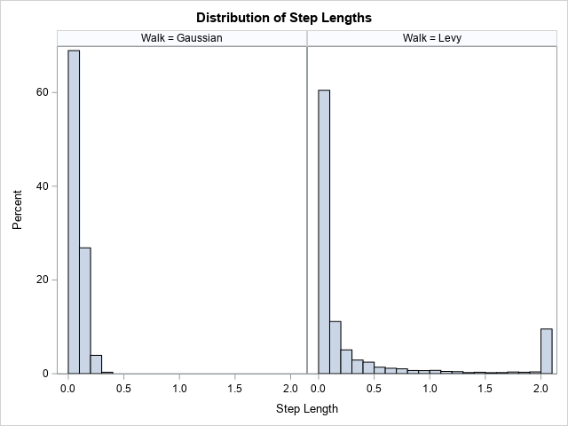
The graph shows that all step lengths for the Gaussian random walk are less than 0.4, which represents four standard deviations for the normal distribution. In contrast, the distribution of distances for the Lévy walk has a long tail. About 15% of the distances are greater than 0.75. About 9% of the step lengths are the maximum possible value, which is 2.

How does that difference affect the amount of territory covered by an animal that is foraging for food? The following statements show the paths of the four animals for each type of random walk:

title "Position of Subjects";
title2 "50 Steps of a Random Walk";
proc sgpanel data=Walks aspect=1;
   where t <= 50;
   panelby Walk / onepanel;
   series x=x y=y / group=Subject;
   colaxis grid; rowaxis grid;
run;

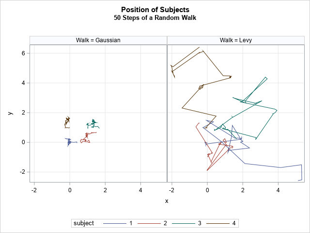
The differences in the paths are evident. For the Gaussian random walk, the simulated animals never leave a small neighborhood around their starting positions. After 50 steps, none of the animals who are taking a Gaussian walk have moved more than one unit away from their starting position. In contrast, the animals who take Lévy walk have explored a much greater region. You can see that the typical motion is several small steps followed by a larger step that brings the animal into a new region to explore.

Generalizing to higher dimensions

It is easy to extend the random walk to higher dimensions. The trick is to represent the "random direction" by a unit vector (u) instead of by an angle (θ). In a previous article about random point within a d-dimensional ball, I remark that "If Y is drawn from the uncorrelated multivariate normal distribution, then u = Y / ||Y|| has the uniform distribution on the unit d-sphere." You can use this trick to generate random unit vectors, then step a distance r in that direction, where r is from a specified distribution of distances.

Summary

An article in Quanta magazine describes how some animals use a swim/flight path that can be modeled by a (truncated) Lévy random walk. This type of movement is a great way to search for food in a vast food-scarce environment. This article defines the Lévy distribution as a sub-family of the inverse gamma distribution. It shows how to generate random variates from the Lévy distribution in SAS. Finally, it simulates a Gaussian random walk and a Lévy walk and visually compares the area explored by each.

Blogs