The inverse gamma distribution is a continuous probability distribution that is used in Bayesian analysis and in some statistical models. The inverse gamma distribution is closely related to the gamma distribution. For any probability distribution, it is essential to know how to compute four functions: the PDF function, which returns the probability density at a given point; the CDF function, which returns the probability that an observation is less than or equal to a particular value; the QUANTILE function, which is the inverse CDF function; and the RAND function, which generates a random variate.

For the gamma distribution, the four essential functions are supported directly in Base SAS. The functions for the inverse gamma distribution are not supported in the same way. However, you can exploit the relationship between the gamma and inverse gamma distributions to implement these four functions for the inverse gamma distribution. This article shows how to implement the PDF, CDF, QUANTILE, and RAND functions for the inverse gamma distribution in SAS.

What is the inverse gamma distribution?

If X is gamma distributed, then X > 0. As its name suggests, the inverse gamma distribution is the distribution of 1/X when X is gamma distributed. More precisely, let Gamma(α, β) be the gamma distribution with shape parameter α and scale parameter β. (This article always uses scale parameters, never a rate parameter.) Let IGamma(α, β) be the inverse gamma distribution with shape and scale parameters. Then if X ~ Gamma(α, β), the random variable 1/X ~ IGamma(α, 1/β). The documentation for PROC MCMC provides an additional discussion of the relationship between the gamma and inverse gamma distributions. There is also a Wikipedia page about the inverse gamma distribution.

A feature of the inverse gamma distribution is that it has a long tail for small values of the α shape parameter. In fact, that the expected value (mean) is undefined when α < 1 and the variance is undefined when α < 2.

Generate random variates from the inverse gamma distribution

It is easy to generate random values from the inverse gamma distribution because that is how the distribution is defined. To obtain a random variate from IGamma(α, β), simply take the reciprocal of a random variate from the Gamma(α, 1/β) distribution. It might be helpful to define a little macro function that makes it easier to generate a random sample. The following SAS program generates a large random sample and displays a histogram:

/* Random values: If X ~ Gamma(alpha, 1/beta), then 1/X ~ IGamma(alpha, beta) */
%macro RandIGamma(alpha, beta);
   (1 / rand('Gamma', &alpha, 1/(&beta)))
%mend;
data IGammaRand;
   call streaminit(12345);
   alpha = 3;
   beta = 0.5;
   do j = 1 to 10000;
      x = %RandIGamma(alpha, beta);
      output;
   end;
run;
 
title "Random Sample from the Inverse Gamma Distribution";
title2 "alpha=3, beta=0.5";
proc sgplot data=IGammaRand noautolegend;
   histogram x / binwidth=0.05 binstart=0.025; 
   xaxis values=(0 to 3 by 0.25);
run;

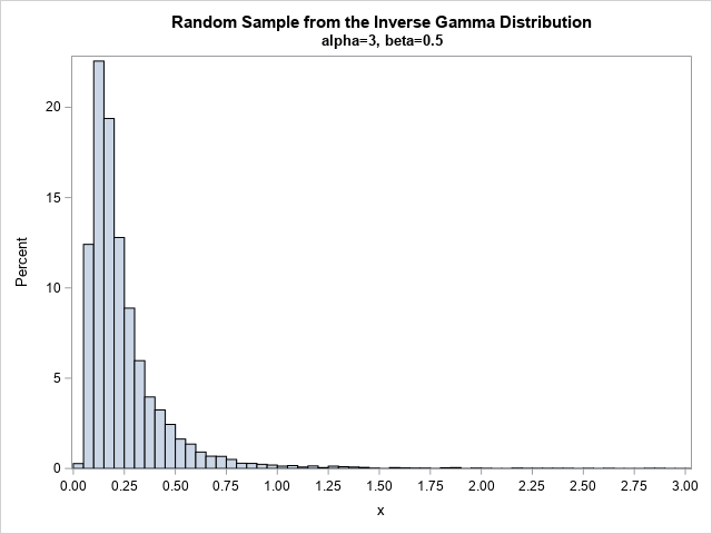
For these values of the parameters, the histogram shows that the distribution has a peak at x=1/8 and a very long tail. The tail is truncated at x=3, but you can use PROC MEANS to see that the maximum value in the sample is 11.69.

The PDF of the inverse gamma distribution

The Wikipedia article gives a formula for the PDF of the inverse gamma article. For x > 0, the PDF formula is
$\mbox{IGamma PDF}(x; \alpha, \beta) = \frac{\beta^{\alpha}}{\Gamma(\alpha)} (1/x)^{\alpha+1} \exp(-\beta/x)$

You can use this relationship to evaluate the inverse gamma PDF in SAS. The following SAS DATA step evaluates the inverse gamma PDF for four choices of (α, β) parameters. These are the same choices that are used in the Wikipedia article for the inverse gamma distribution.

/* PDF : parameterize IGamma by using the scale parameter
   in terms of the Gamma PDF with shape parameter. */
%macro PDFIGamma(x, alpha, beta);
   (pdf("Gamma", 1/(&x), &alpha, 1/(&beta)) / ((&x)**2))
%mend;
 
data IGammaPDF;
array a[4] _temporary_ (1 2 3 3);
array b[4] _temporary_ (1 1 1 0.5);
do i = 1 to dim(a);
   alpha = a[i];
   beta  = b[i];
   group = cat('a=',alpha,', b=',beta);
   do x = 0.01 to 3 by 0.01;
      pdf = %PDFIGamma(x, alpha, beta);
      /* equivalent to 
      pdf = beta**alpha / Gamma(alpha) * x**(-alpha-1) * exp(-beta/x); */
      output;
   end;
end;
run;
 
title "PDF of the Inverse Gamma Distribution";
proc sgplot data=IGammaPDF;
   series x=x y=PDF / group=group lineattrs=(thickness=2);
   xaxis grid label="Density"; yaxis grid;
run;

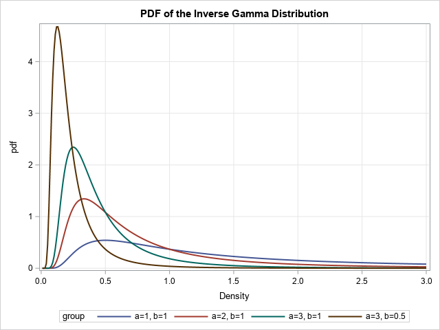
You can see that the brown curve (the PDF for (α, β) = (3, 0.5)) has the same shape as the histogram of the random sample in the previous section.

The CDF and quantiles of the inverse gamma distribution

In a previous article, I show that there is a relationship between the CDF of the gamma distribution and a special function called the regularized upper incomplete gamma function. I also show how to compute the incomplete gamma function in SAS. In Wikipedia, the CDF of the inverse gamma distribution is given in terms of the incomplete gamma function. Consequently, we can compute the CDF in SAS without difficulty.

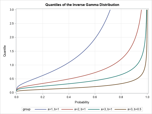
The quantile function is more difficult. The quantile function is the inverse CDF. There are a LOT of reciprocals to keep track of during the derivation! Nevertheless, you can evaluate the quantile function of the inverse gamma distribution by using an expression that includes the quantile function of the gamma distribution. The derivation is left as an exercise.

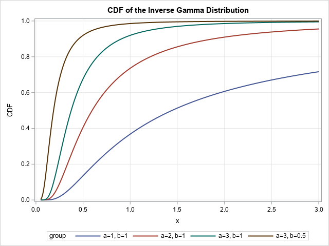
The following DATA step evaluates the CDF of the inverse gamma distribution for four sets of parameters. The quantile function is evaluated at the same time to ensure that Quantile(CDF(x)) = x. The CDF function is very flat for very small values of x, so the quantile function might fail to converge for very small values of the probability.

/* The CDF of the IGAMMA function is SDF('Gamma',1/x,alpha,1/beta) */
%macro CDFIGamma(x, alpha, beta);
   (SDF('Gamma', (&beta)/(&x), &alpha))
%mend;
%macro QuantileIGamma(p, alpha, beta);
   (1 / quantile('Gamma', 1-(&p), &alpha, 1/(&beta)))
%mend;
 
data IGammaCDF;
array a[4] _temporary_ (1 2 3 3);
array b[4] _temporary_ (1 1 1 0.5);
do i = 1 to dim(a);
   alpha = a[i];
   beta  = b[i];
   group = cat('a=',alpha,', b=',beta);
   do x = 0.05 to 3 by 0.01;
      CDF = %CDFIGamma(x, alpha, beta); 
      Quantile = %QuantileIGamma(CDF, alpha, beta); /* x - Quantile is approx 0 */
      output;
   end;
end;
run;
 
title "CDF of the Inverse Gamma Distribution";
proc sgplot data=IGammaCDF;
   series x=x y=CDF / group=group lineattrs=(thickness=2);
   xaxis grid; yaxis grid;
run;
 
title "Quantiles of the Inverse Gamma Distribution";
proc sgplot data=IGammaCDF;
   series x=CDF y=Quantile / group=group lineattrs=(thickness=2);
   xaxis grid label="Probability"; yaxis grid;
run;

Summary

This article shows how to compute the four essentials functions of the inverse gamma distribution: random variates, PDF, CDF, and quantiles. In every case, you can exploit the relationship between the gamma and inverse gamma distributions. The result is that you can use the RAND, PDF, CDF, and QUANTILE functions for the gamma distribution to evaluate similar quantities for the inverse gamma distribution. A contribution of this article is to write down the four formulas in one place and show how to compute them in SAS.