When working with a probability distribution, it is useful to know how to compute four essential quantities: a random sample, the density function, the cumulative distribution function (CDF), and quantiles. I recently discussed the Poisson-binomial distribution and showed how to generate a random sample. This article shows how to compute the PDF for the Poisson-binomial distribution. From the PDF function, you can quickly compute the cumulative distribution (CDF) and the quantile function. For a discrete distribution, the PDF is also known as the probability mass function (PMF).

In a 2013 paper, Y. Hong describes several ways to compute or approximate the PDF for the Poisson-binomial distribution. This article uses SAS/IML to implement one of the recurrence formulas (RF1, Eqn 9) in his paper. Hong attributes this formula to Barlow and Heidtmann (1984). A previous article discusses how to compute recurrence relations in SAS.

A recurrence relation for the Poisson-binomial PDF

You can read my previous article or the Chen (2013) paper to learn more about the Poisson-binomial (PB) distribution. The PB distribution is generated by running N independent Bernoulli trials, each with its own probability of success. These probabilities are the N parameters for the PB distribution: p1, p2, ..., pN.

A PB random variable is the number of successes among the N trials, which will be an integer in the range [0, N]. If X is a PB random variable, the PDF is the probability of observing k successes for k=0,1,...,N. That is, PDF(k) = Pr[X=k]. This probability depends on the N probabilities for the underlying Bernoulli trials.

If you are not interested in how to compute the PDF from a recurrence relation, you can skip to the next section.

Let's assume that we always perform the Bernoulli trials in the same order. (They are independent trials, so the order doesn't matter.) Define ξ[k,j] to be the probability that k successes are observed after performing the first j trials, 0 ≤ k,j ≤ N. Note that PDF(k) = ξ[k,N].

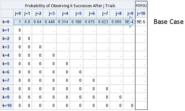
As mentioned earlier, we will use a recurrence relation to compute the PDF for each value of k=0,1,...,N. If you picture the ξ array as a matrix, you can put zeros for all the probabilities in the lower triangular portion of the matrix because the probability of observing j successes is zero if you have performed fewer than j trials.

You can also fill in the first row of the matrix, which is the probability of observing k=0 successes. The only way that you can observe zero successes after j trials is if no trial was a success. Because the trials are independent, the probability is the product Π (1-p[i]), where the product is over i=1..j. This enables us to fill in the top row of the ξ matrix. Consequently, PDF(0) is the product of 1-p[i]over all i=1..N. After completing the first row (the base case), the ξ matrix looks like the following:

The recurrence relation for filling in the table is given by the formula
ξ[k, j] = (1-p[j])*ξ[k,j-1] + p[j]*ξ[k-1,j]
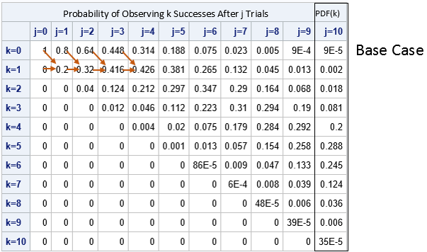
This formula enables you to compute the k_th row (starting at the left side) provided that you know the values of the (k-1)st row. A cell in the matrix can be computed if you know the value of the cell in the previous column for that row and for the previous row. The following diagram show this idea. The arrows in the row for k=1 indicate that you can compute those cells from left to right. First, you compute ξ[1, 1], then ξ[1, 2], then ξ[1, 3], and so forth. When you reach the end of the row, you have computed PDF(1). You then fill in the next row (from left to right) and continue this process until all cells are filled.

You can understand the recurrence relation in terms of the underlying Bernoulli trials. Suppose you have already performed j-1 trials, are getting ready to perform the j_th. There are two situations for which the j_th trial will produce the k_th success:

• The first j-1 trials produced k successes and the j_th trial is a failure. This happens with probability (1-p[j])*ξ[k,j-1], which is the first term in the recurrence relation.
• The first j-1 trials produced k-1 successes and the j_th trial is a success. This happens with probability p[j]ξ[k-1,j], which is the second term in the recurrence relation.

Although I have displayed the entire ξ matrix, I will point out that you do not need to store the entire matrix. You can compute each row by knowing only the previous row. This seems to have been overlooked by Hong, who remarked that the "RF1 method can be computer memory demanding when N is large" (p. 8) and "when N = 15,000, approximately 4GB memory is needed for computing the entire CDF." Neither of those statements is true. You only need two arrays of size N, and the required RAM for two arrays of size N = 15,000 is 0.22 MB (or 2.2E-4 GB).

Compute the Poisson-binomial PDF in SAS

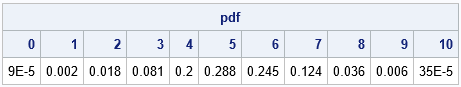
You can use the SAS/IML language to implement the recurrence formula. The following program uses N=10 and the same vector of probabilities as in the previous article.

proc iml;
start PDFPoisBinom(_p);
   p = colvec(_p); N = nrow(p);
   R = j(1, N+1, 0);        /* R = previous row of probability matrix */
   S = j(1, N+1, 0);        /* S = current row of probability matrix */
   R[1] = 1;
   R[2:N+1] = cuprod(1-p);  /* first row (k=0) is cumulative product */
   pdf0 = R[N+1];           /* pdf(0) is last column of row */ 
   pdf = j(1, N);
   do k = 1 to N;           /* for each row k=1..N */
      S[,] = 0;             /* zero out the current row */
      do j = k to N;        /* apply recurrence relation from left to right */
         S[j+1] = (1-p[j])*S[j] + p[j]*R[j];  
      end;
      pdf[k] = S[N+1];      /* pdf(k) is last column of row */
      R = S;                /* store this row for the next iteration */
   end;
   return (pdf0 || pdf);    /* return PDF as a row vector */
finish;
 
p = {0.2, 0.2, 0.3, 0.3, 0.4, 0.6, 0.7, 0.8, 0.8, 0.9};  /* 10 trials */
pdf = PDFPoisBinom(p);
print pdf[c=('0':'10') F=Best5.];

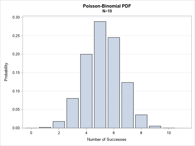
You can use PROC SGPLOT to create a bar chart that visualizes the PDF:

Compute the Poisson-binomial CDF

For a discrete distribution, you can easily compute the CDF and quantiles from the PDF. The CDF is merely the cumulative sum of the PDF values. You can use the CUSUM in SAS/IML to compute a cumulative sum, so the SAS/IML function that computes the CDF is very short:

start CDFPoisBinom(p);
   pdf = PDFPoisBinom(p);
   return ( cusum(pdf) );   /* The CDF is the cumulative sum of the PDF */
finish;
 
cdf = CDFPoisBinom(p);
print cdf[c=('0':'10') F=Best5.];

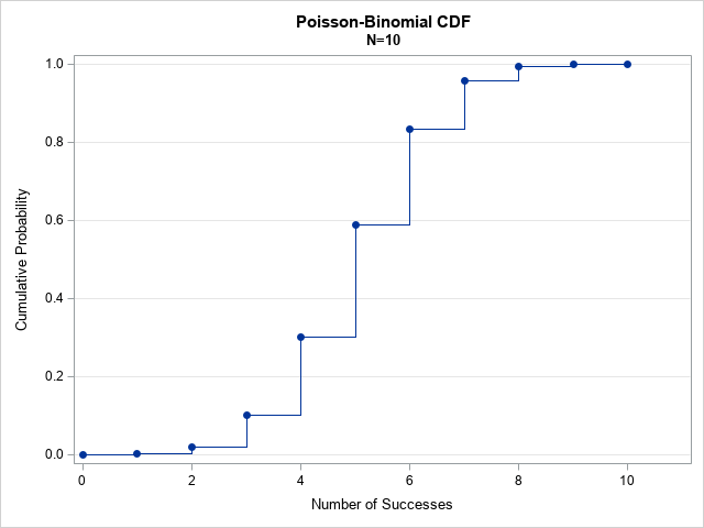
Instead of displaying the table of values, I have displayed the CDF as a graph. I could have used a bar chart or needle plot, but I chose to visualize the CDF as a step function because that representation is helpful for computing quantiles, as shown in the next section.

Compute the Poisson-binomial quantiles

Given a probability, ρ, the quantile for a discrete distribution is the smallest value for which the CDF is greater than or equal to ρ. The quantile function for the Poisson-binomial distribution is a value, q, in the range [0, N]. Geometrically, you can use the previous graph to compute the quantiles: Draw a horizontal line at height ρ and see where it crosses a vertical line on the CDF graph. That vertical line is located at the value of the quantile for ρ. The following SAS/IML module implements the quantile function:

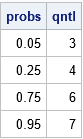
/* The quantile is the smallest value for which the CDF is greater than or equal to 
   the given probability. */
start QuantilePoisBinom(p, _probs);        /* p = PB parameters; _prob = vector of probabilities for quantiles */
   cdf = CDFPoisBinom(p);                  /* index is one-based */
   probs = colvec(_probs);                 /* find quantiles for these probabilities */
   q = j(nrow(probs), 1, .);               /* allocate result vector */
   do i = 1 to nrow(probs);
      idx = loc( probs[i] <= CDF );        /* find all x such that p <= CDF(x) */ 
      q[i] = idx[1] - 1;                   /* smallest index. Subtract 1 b/c PDF is for k=0,1,...,N  */
   end;
   return ( q );
finish;
 
probs = {0.05, 0.25, 0.75, 0.95};
qntl = QuantilePoisBinom(p, probs);
print probs qntl;

Summary

By using a recurrence relation, you can compute the entire probability density function (PDF) for the Poisson-binomial distribution. From those values, you can obtain the cumulative distribution (CDF). From the CDF, you can obtain the quantiles. This article implements SAS/IML functions that compute the PDF, CDF, and quantiles. A previous article shows how to generates a random sample from the Poisson-binomial distribution.

You can download the complete SAS program that computes the quantities and creates the graphs in this article.

References

Hong, Y., (2013) "On computing the distribution function for the Poisson binomial distribution," Computational Statistics & Data Analysis, 59:41–51.