Many textbooks and research papers present formulas that involve recurrence relations. Familiar examples include:

• The factorial function: Set Fact(0)=1 and define Fact(n) = n*Fact(n-1) for n > 0.
• The Fibonacci numbers: Set Fib(0)=1 and Fib(1)=1 and define Fib(n) = Fib(n-1) + Fib(n-2) for n > 1.
• The binomial coefficients (combinations of "n choose k"): For a set that has n elements, set Comb(n,0)=1 and Comb(n,n)=1 and define Comb(n,k) = Comb(n-1, k-1) + Comb(n-1, k) for 0 ≤ k ≤ n.
• Time series models: In many time series models (such as the ARMA model), the response and error terms depend on values at previous time points. This leads to recurrence relations.

Sometimes the indices begin at 0, other times they begin at 1. Working efficiently with sequences and recurrence relations can be a challenge. The SAS DATA step is designed to processes one observation at a time, but a recurrence relation requires looking at past values. If you use the SAS DATA step to work with recurrence relations, you need to use tricks to store and refer to previous values. Another challenge is indexing: most SAS programmers are used to one-based indexing, whereas some formulas use zero-based indexing.

This article uses the Fibonacci numbers to illustrate how to deal with some of these issues in SAS. There are several definitions of the Fibonacci numbers, but we'll look at the definition that uses zero indexing: F₀ = 1, F₁ = 1, and F_n = F_n-1 + F_n-2 for n > 1. In this article, I will use n ≤ 7 to demonstrate the concepts.

Recurrence relations by using arrays

The SAS DATA step supports arrays, and you can specify the indices of the arrays. Therefore, you can specify that an array index starts with zero. The following DATA step generates "wide" data. There is one observation, and the variables are named F0-F7.

data FibonacciWide;
array F[0:7] F0-F7;  /* index starts at 0 */
F[0] = 1;            /* initialize first values */
F[1] = 1;
do i = 2 to 7;       /* apply recurrence relation */
   F[i] = F[i-1] + F[i-2];
end;
drop i;
run;
 
proc print noobs; run;

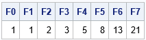
You can mentally check that each number is the sum of the two previous numbers. Using an array is convenient and easy to program. Unfortunately, this method is not very useful in practice. In practice, you usually want the data in long form rather than wide form. For example, if you simulate time series data, each observation represents a time point and the values depend on previous time points.

Recurrence relations by using extra variables

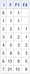
In the DATA step, you can use the concept of "lags" to implement a recurrence relation. A lag is any previous value. If we are currently computing the n_th value, the first lag is the (n-1)th value, which is the previous observation. The second lag is the (n-2)th value and so forth. One way to look at previous values is to save them in an extra variable. The following DATA step uses F1 to hold the first lag of F and F2 to hold the second lag of F. Recall that the SUM function will return the sum of the nonmissing values, so sum(F1, F2) is nonmissing if F1 is nonmissing.

data FibonacciLong;
F1 = 1; F2 = .;        /* initialize lags */
i=0; F = F1; output;   /* manually output F(0) */
do i = 1 to 7;         /* now iterate: F(i) = F(i-1) + F(i-2) */
   F = sum(F1, F2);
   output;
   F2 = F1;            /* update lags for the next iteration */
   F1 = F;
end;
run;
 
proc print noobs; 
   var i F F1 F2; 
run;

Recurrence relations by using the LAG function

The DATA step supports a LAGn function. The LAGn function maintains a queue of length n, which initially contains missing values. Every time you call the LAGn function, it pops the top of the queue, returns that value, and adds the current value of its argument to the end of the queue. The LAGn functions can be surprisingly difficult to use in a complicated program because the queue is only updated when the function is called. If you have conditional IF-THEN/ELSE logic, you need to be careful to keep the queues up to date. I confess that I am often frustrated when I try to use the LAG function with recurrence relations. I find it easier to use extra variables.

But since the documentation for the LAGn function includes the Fibonacci numbers among its examples, I include it here. Notice the clever use of calling LAG1(F) and immediately assigning the new value of F, so that the program only needs to compute the first lag and does not use any extra variables:

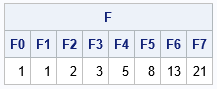
/* modified from documentation for the LAG function */
data FibonacciLag;
i=0; F=1; output;       /* initialize and output F[0] */
/* lag1(F) is missing when _N_=1, but equals F[i-1] in later iters */
do i = 1 to 7;
   F = sum(F, lag(F));  /* iterate: F(i) = F(i-1) + F(i-2) */
   output;
end;
run;
 
proc print noobs; run;

The values are the same as for the previous program, but notice that this program does not use any extra variables to store the lags.

Recurrence relations in SAS/IML

Statistical programmers use the SAS/IML matrix language because of its power and flexibility, but also because you can vectorize computations. A vectorized computation is one in which an iterative loop is replaced by a matrix-vector computation. Unfortunately, for many time series computations, you cannot completely get rid of the loops because the series is defined in terms of a recurrence relation. You cannot compute the n_th value until you have computed the previous values.

The easiest way to implement a recurrence relation in the SAS/IML language is to use the DATA step program for generating the "wide form" sequence. The PROC IML code is almost identical to the DATA step code:

proc iml;
N = 8;
F = j(1, N, 1);            /* initialize F[1]=F[2]=1 */
do i = 3 to N;             
   F[i] = F[i-1] + F[i-2]; /* overwrite F[i] with the sum of previous terms, i > 2 */
end;
labls = 'F0':'F7';
print F[c=labls];

The program is efficient and straightforward. The output is not shown. The SAS/IML language does not support 0-based indexing, so for recurrence relations that start at 0, I usually define the indexes to match the recurrence relation and add 1 to the subscripts of the IML vectors. For example, if you index from 0 to 7 in the previous program, the body of the loop becomes F[i+1] = F[i]+ F[i-1].

Linear recurrence relations and matrix iteration

The Fibonacci sequence is an example of a linear recurrence relations. For a linear recurrence relation, you can use matrices and vectors to generate values. You can define the Fibonacci matrix to be the 2 x 2 matrix with values {0 1, 1 1}. The Fibonacci matrix transforms a vector {x1, x2} into the vector {x2, x1+x2}. In other words, it moves the second element to the first element and replaces the second element with the sum of the elements. If you iterate this transformation, the iterates generate the Fibonacci numbers, as shown in the following statements:

M = {0 1,                  /* Fibonacci matrix */
     1 1};
v = {1, 1};                /* initial state */
F = j(1, N, 1);            /* initialize F[1]=1 */
do i = 2 to N;             
   v = M*v;                /* generate next Fibonacci number */
   F[i] = v[1];            /* save the number in an array */
end;
print F[c=labls];

You can use this method to generate sequences in any linear recurrence relation. Previous methods work for linear or nonlinear recurrence relationships. The SAS/IML language also supports a LAG function, although it works differently from the DATA step function of the same name.

Summary

This article shows a few ways to work with recurrence relations in SAS. You can use DATA step arrays to apply relations for "wide form" data. You can use extra variables or the LAG function for long form data. You can perform similar computations in PROC IML. If the recurrence relation is linear, you can also use matrix-vector computations to apply each step of the recurrence relation.