The Poisson-binomial distribution is a generalization of the binomial distribution.

• For the binomial distribution, you carry out N independent and identical Bernoulli trials. Each trial has a probability, p, of success. The total number of successes, which can be between 0 and N, is a binomial random variable. The distribution of that random variable is the binomial distribution.
• The Poisson-binomial distribution is similar, but the probability of success can vary among the Bernoulli trials. That is, you carry out N independent but not identical Bernoulli trials. The j_th trial has a probability, p_j, of success. The total number of successes, which can be between 0 and N, is a random variable. The distribution of that random variable is the Poisson-binomial distribution.

This article shows how to generate a random sample from the Poisson-binomial distribution in SAS. Simulating a random sample is a great way to begin exploring a new distribution because the empirical density and empirical cumulative distribution enable you to see the shape of the distribution and how it depends on parameters.

Generate a random binomial sample

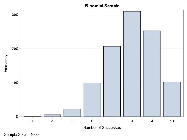
Before looking at the Poisson-binomial distribution, let's review the more familiar binomial distribution. The binomial distribution has two parameters: the probability of success (p) and the number of Bernoulli trials (N). The output from a binomial distribution is a random variable, k. The random variable is an integer between 0 and N and represents the number of successes among the N Bernoulli trials. If you perform many draws from the binomial distribution, the sample will look similar to the underlying probability distribution, which has mean N*p and variance N*p*(1-p).

SAS supports sampling from the binomial distribution by using the RAND function. The following SAS DATA step generates a random sample of 1,000 observations from the binomial distribution and plots the distribution of the sample:

/* Generate a random sample from the binomial distribution */
/* The Easy Way: call rand("Binom", p, N) */
%let m = 1000;              /* number of obs in random sample */
data BinomSample;
call streaminit(123);
p = 0.8; N = 10;            /* p = prob of success; N = num trials */
label k="Number of Successes";
do i = 1 to &m;
   k = rand("Binom", p, N); /* k = number of successes in N trials */
   output;
end;
keep i k;
run;
 
title "Binomial Sample";
footnote J=L "Sample Size = &m";
proc sgplot data=BinomSample;
   vbar k;
   yaxis grid;
run;

This is the standard way to generate a random sample from the binomial distribution. In fact, with appropriate modifications, this program shows the standard way to simulate a random sample of size m from ANY of the built-in probability distributions in SAS.

Another way to simulate binomial data

Let's pretend for a moment that SAS does not support the binomial distribution. You could still simulate binomial data by making N calls to the Bernoulli distribution and counting the number of successes. The following program generates a binomial random variable by summing the results of N Bernoulli random variables:

/* The Alternative Way: Make N calls to rand("Bernoulli", p) */
data BinomSample2(keep=i k);
call streaminit(123);
p = 0.8; N = 10;
label k="Number of Successes";
do i = 1 to &m;
   k = 0;                            /* initialize k=0 */
   do j = 1 to N;                    /* sum of N Bernoulli variables */
      k = k + rand("Bernoulli", p);  /* every trial has the same probability, p */
   end;
   output;
end;
run;

The output data set is also a valid sample from the Binom(p, N) distribution. The program shows that you can replace the single call to RAND("Binom",p,N) with N calls to RAND("Bernoulli",p). You then must add up all the binary (0 or 1) random variables from the Bernoulli distribution.

Simulate Poisson-binomial data

The program in the previous section can be modified to generate data from the Poisson-binomial distribution. Instead of using the same probability for all Bernoulli trials, you can define an array of probabilities and use them to generate the Bernoulli random variables. This is shown by the following program, which generates the number of successes in a sequence of 10 Bernoulli trials where the probability of success varies among the trials:

/* generate a random sample from the Poisson-binomial distribution 
   that has 10 parameters: p1, p2, p3, ..., p10 */
data PoisBinomSample(keep=i k);
/* p[j] = probability of success for the j_th trial, i=1,2,...,10 */
array p[10] (0.2 0.2 0.3 0.3 0.4 0.6 0.7 0.8 0.8 0.9);  /* N = dim(p) */
call streaminit(123);
label k="Number of Successes";
do i = 1 to &m;
   k = 0;                              /* initialize k=0 */
   do j = 1 to dim(p);                 /* sum of N Bernoulli variables */
      k = k + rand("Bernoulli", p[j]); /* j_th trial has probability p[j] */
   end;
   output;
end;
run;
 
title "Poisson-Binomial Sample";
proc sgplot data=PoisBinomSample;
   vbar k;
   yaxis grid;
run;

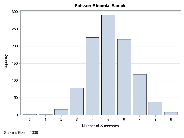
The graph shows the distribution of a Poisson-binomial random sample. Each observation in the sample is the result of running the 10 trials and recording the number of successes. You can see from the graph that many of the trials resulted in 5 successes, although 4 or 6 are also very likely. For these parameters, it is rare to see 0 or 1 success, although both occurred during the 1,000 sets of trials. Seeing 10 successes is mathematically possible but did not occur in this simulation.

In this example, the vector of probabilities has both high and low probabilities. The probability of success is 0.2 for one trial and 0.9 for another. If you change the parameters in the Poisson-binomial distribution, you can get distributions that have different shapes. For example, if all the probabilities are small (close to zero), then the distribution will be positively skewed and the probability of seeing 0, 1, or 2 successes is high. Similarly, if all the probabilities are large (close to one), then the distribution will be negatively skewed and there is a high probability of seeing 8, 9, or 10 successes. If all probabilities are equal, then you get a binomial distribution.

Simulate Poisson-binomial data by using SAS/IML

The SAS/IML language makes it easy to encapsulate the Poisson-binomial simulation into a function. The function has two input arguments: the number of observations to simulate (m) and the vector of probabilities (p). The output of the function is a vector of m integers. For example, the following SAS/IML function implements the simulation of Poisson-binomial data:

proc iml;
/* Simulate from the Poisson-Binomial distribution. 
   Input: m = number of observations in sample
          p = column vector of N probabilities. The probability 
              of success for the j_th Bernoulli trial is p_j.
   Output: row vector of m realizations of X ~ PoisBinom(p) 
*/
start RandPoisBinom(m, _p);
   p = colvec(_p);
   b = j(nrow(p), m);     /* each column is a binary indicator var */
   call randgen(b, "Bernoulli", p); 
   return( b[+, ] );      /* return numSuccesses = sum each column */
finish;
 
/* The Poisson-binomial has N parameters: p1, p2, ..., pN */
p = {0.2 0.2 0.3 0.3 0.4 0.6 0.7 0.8 0.8 0.9};  /* 10 trials */
call randseed(123);
S = RandPoisBinom(&m, p);
call bar(S) grid="y" label="Number of Successes";

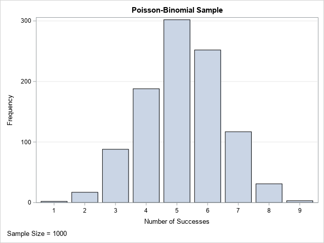
The SAS/IML program uses the RANDGEN function to fill up an N x m matrix with values from the Bernoulli distribution. The RANDGEN function supports a vector of parameters, which means that you can easily specify that each column should have a different probability of success. After filling the matrix with binary values, you can use the summation subscript reduction operator to obtain the number of successes (1s) in each column. The result is a row vector that contains m integers, each of which is the number of successes from a set of N Bernoulli trials with the given probabilities.

The PROC IML program uses the same parameters as the DATA step simulation. Accordingly, the sample distributions are similar.

The expected value of the Poisson-binomial distribution is the sum of the vector of probabilities. The variance is the sum of the individual Bernoulli variances. You can compute the mean and variance of the distribution and compare it to the sample mean and variance:

/* Expected values: mean and variance of the Poisson-binomial distribution */
mu = sum(p);
var = sum( (1-p)#p );
/* sample estimates of mean and variance */
XBar = mean(S`);
s2 = var(S`);
Moments = (mu//XBar) || (var//s2);
print Moments[f=5.2 r={"Distribution" "Sample Estimate"} c={"Mean" "Variance"}];

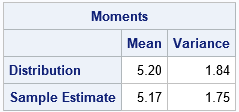
The expected number of successes in the Poisson-binomial distribution with these parameters is 5.2. In the sample, the average number of successes is 5.17. The variance of the Poisson-binomial distribution is 1.84. The variance of this sample is 1.75. The sample statistics are close to their expected values, which is what you expect to happen for a large random sample.

Summary

This article shows how to simulate data from the Poisson-binomial distribution. A random variable that follows the Poisson-binomial distribution gives the total number of success in N Bernoulli trials, where the j_th trial has the probability p_j of success. The example in this article uses a 10-parameter vector of probabilities. If all parameter values are identical (p), then the Poisson-binomial distribution reduces to the standard Binom(p, 10) distribution. However, the Poisson-binomial distribution allows the probabilities to be different.

You can download the SAS program that computes the quantities and creates the graphs in this article.