I recently showed how to use linear interpolation in SAS. Linear interpolation is a common way to interpolate between a set of planar points, but the interpolating function (the interpolant) is not smooth. If you want a smoother interpolant, you can use cubic spline interpolation. This article describes how to use a cubic spline interpolation in SAS.

As mentioned in my previous post, an interpolation requires two sets of numbers:

1. Data: Let (x1, y1), (x2, y2), ..., (xn, yn) be a set of n data points. These sample data should not contain any missing values. The data must be ordered so that x1 < x2 < ... < xn.
2. Values to score: Let {t1, t2, ..., tk} be a set of k new values for the X variable. For interpolation, all values must be within the range of the data: x1 ≤ t_i ≤ xn for all i. The goal of interpolation is to produce a new Y value for each value of t_i. The scoring data is also called the "query data."

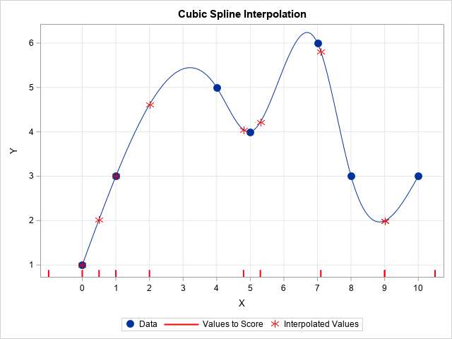
The following SAS DATA steps define the data for this example. The POINTS data set contains the sample data, which are shown as blue markers on the graph to the right. The SCORE data set contains the scoring data, which are shown as red tick marks along the horizontal axis.

/* Example dats for 1-D interpolation */
data Points;  /* these points define the model */
input x y;
datalines;
0  1
1  3
4  5
5  4
7  6
8  3
10 3
;
 
data Score; /* these points are to be interpolated */
input t @@;
datalines;
2 -1 4.8 0 0.5 1 9 5.3 7.1 10.5 9
;

On the graph, the blue curve is the cubic spline interpolant. Every point that you interpolate will be on that curve. The red asterisks are the interpolated values for the values in the SCORE data set. Notice that points -1 and 10.5 are not interpolated because they are outside of the data range. The following section shows how to compute the cubic spline interpolation in SAS.

Cubic spline interpolation in SAS

A linear interpolation uses a linear function on each interval between the data points. In general, the linear segments do not meet smoothly: the resulting interpolant is continuous but not smooth. In contrast, spline interpolation uses a polynomial function on each interval and chooses the polynomials so that the interpolant is smooth where adjacent polynomials meet. For polynomials of degree k, you can match the first k – 1 derivatives at each data point.

A cubic spline is composed of piecewise cubic polynomials whose first and second derivatives match at each data point. Typically, the second derivatives at the minimum and maximum of the data are set to zero. This kind of spline is known as a "natural cubic spline" with knots placed at each data point.

I have previously shown how use the SPLINE call in SAS/IML to compute a smoothing spline. A smoothing spline is not an interpolant because it does not pass through the original data points. However, you can get interpolation by using the SMOOTH=0 option. Adding the TYPE='zero' option results in a natural cubic spline.

For more control over the interpolation, you can use the SPLINEC function ('C' for coefficients) to fit the cubic splines to the data and obtain a matrix of coefficients. You can then use that matrix in the SPLINEV function ('V' for value) to evaluate the interpolant at the locations in the scoring data.

The following SAS/IML function (CubicInterp) computes the spline coefficients from the sample data and then interpolates the scoring data. The details of the computation are provided in the comments, but you do not need to know the details in order to use the function to interpolate data:

/* Cubic interpolating spline in SAS.
   The interpolation is based on the values (x1,y1), (x2,y2), ..., (xn, yn).
   The X  values must be nonmissing and in increasing order: x1 < x2 < ... < xn
   The values of the t vector are interpolated.
*/
proc iml;
start CubicInterp(x, y, t);
   d = dif(x, 1, 1);                     /* check that x[i+1] > x[i] */
   if any(d<=0) then stop "ERROR: x values must be nonmissing and strictly increasing.";
   idx = loc(t>=min(x) && t<=max(x));    /* check for valid scoring values */
   if ncol(idx)=0 then stop "ERROR: No values of t are inside the range of x.";
 
   /* fit the cubic model to the data */
   call splinec(splPred, coeff, endSlopes, x||y) smooth=0 type="zero";
 
   p = j(nrow(t)*ncol(t), 1, .);       /* allocate output (prediction) vector */
   call sortndx(ndx, colvec(t));       /* SPLINEV wants sorted data, so get sort index for t */
   sort_t = t[ndx];                    /* sorted version of t */
   sort_pred = splinev(coeff, sort_t); /* evaluate model at (sorted) points of t */
   p[ndx] = sort_pred[,2];             /* "unsort" by using the inverse sort index */
   return( p );
finish;
 
/* example of linear interpolation in SAS */
use Points; read all var {'x' 'y'}; close;
use Score; read all var 't'; close;
 
pred = CubicInterp(x, y, t);
create PRED var {'t' 'pred'}; append; close;
QUIT;

The visualization of the interpolation is similar to the code in the previous article, so the code is not shown here. However, you can download the SAS program that performs the cubic interpolation and creates the graph at the top of this article.

Although cubic spline interpolation is slower than linear interpolation, it is still fast: The CubicInterp program takes about 0.75 seconds to fit 1000 data points and interpolate one million scoring values.

Summary

In summary, the SAS/IML language provides the computational tools for cubic spline interpolation. The CubicInterp function in this article encapsulates the functionality so that you can perform cubic spline interpolation of your data in an efficient manner.