I've previously written about how to generate points that are uniformly distributed in the unit disk. A seemingly unrelated topic is the distribution of eigenvalues (in the complex plane) of various kinds of random matrices. However, I recently learned that these topics are somewhat related!

A mathematical result called the "Circular Law" states that the (complex) eigenvalues of a (scaled) random n x n matrix are uniformly distributed in a disk as n → ∞. For this article, a random matrix is one whose entries are independent random variates from a specified distribution that has mean 0 and unit variance. A more precise statement of the circular law is found in the link, but, loosely speaking, if A_n is a sequence of random matrices of increasing size, the distribution of the eigenvalues of (1/sqrt(n)) A_n converges to the uniform distribution in the unit disk as n → ∞.

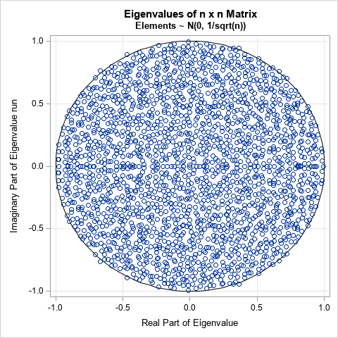
This article uses SAS to visualize the eigenvalue of several large random matrices. The graph to the right shows the complex eigenvalues for an n x n matrix whose entries are normal random variates from N(0, 1/sqrt(n)), where n = 2000. These eigenvalues appear to be uniformly distributed, as the circular law dictates, and most are inside the unit disk.

To demonstrate the circular law, you can fill a large n x n matrix with independent variates from any probability distribution that has mean 0 and unit variance. The matrix is then scaled by dividing each entry by sqrt(n). Equivalently, you can save a step and fill the matrix with random variates from a distribution that has 0 mean and standard deviation 1/sqrt(n).

Eigenvalues of random matrices

Let me be perfectly clear: There are simple and efficient algorithms to simulate uniformly distributed variates in the unit disk. No one should use the eigenvalue of a large matrix as a way to simulate uniform variates in a disk!

The following SAS/IML program creates a random 2000 x 2000 matrix where each element is a random variate from the N(0, 1/sqrt(n)) distribution, which has mean 0 and standard deviation 1/sqrt(n). It then computes the eigenvalues (which are complex) and writes them to a data set. Because I intend to repeat these computations for other distributions, I use a macro variable (DSName) to hold the name of the variable and I use a macro (RandCall) to specify the IML statement that fills a matrix, M, with random variates:

/* Demonstrate the circular law: eigenvalues are uniform in unit disk */
title "Eigenvalues of n x n Matrix";
 
/* title, data set name, and IML statement for a distribution */
title2 "Elements ~ N(0, 1/sqrt(n))";
%let DSName = Normal;
%macro RandCall;
   call randgen(M, "Normal", 0, 1/sqrt(n));
%mend;
 
proc iml;
call randseed(12345);
n = 2000;                            /* sample size = dim of matrix */
M = j(n, n);
%RandCall;
v = eigval(M);
create &DSName from v[c={"Re" "Im"}]; append from v; close; 
quit;

To visualize the eigenvalues, you can create a scatter plot that displays the real part (Re) and the imaginary part (Im) of each eigenvalue. I want to overlay a unit circle on the graph, so the following DATA step creates a piecewise linear approximation of a circle and uses the POLYGON statement in PROC SGPLOT to overlay the eigenvalues and the circle:

data Circle;
retain ID 1  k 100;
pi = constant('pi');
do theta = 0 to 2*pi by 2*pi/k;
   px = cos(theta);   py = sin(theta);   output;
end;
keep ID px py;
run;
 
data All;
set &DSName Circle;
label Re = "Real Part of Eigenvalue"
      Im = "Imaginary Part of Eigenvalue"
run;
 
ods graphics / width=480px height=480px;
proc sgplot data=All aspect=1 noautolegend;
   polygon x=px y=py ID=ID;   /* the unit circle */
   scatter x=Re y=Im;         /* the complex eigenvalues */
   xaxis grid; yaxis grid;
quit;

The graph is shown at the top of this article. It certainly appears that the eigenvalues of the 2000 x 2000 matrix are uniformly distributed. However, if you look carefully, a few eigenvalues appear to be outside of the unit disk. You can compute the distance from the origin for each eigenvalue (Re² + Im²) and compare that distance to 1 to count how many of the 2000 eigenvalues are outside the unit circle:

data InOut;
set &DSName;
InDisk = (Re**2 + Im**2 <= 1);   /* indicator variable */
run;
 
proc freq data=InOut order=freq;
   tables InDisk / nocum ;
run;

For this random matrix, 12 eigenvalues are not inside the unit disk. Thus, although the eigenvalues appear to be approximately uniformly distributed, it is only in the limit as n → ∞ that all eigenvalues are inside the closed disk.

Other probability distributions

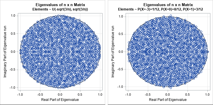
The remarkable thing about the circular law is that it is true for ANY probability distribution that has mean 0 and standard deviation 1/sqrt(n). To demonstrate, you can graph the eigenvalues for matrices that are filled with random variates from two other probability distributions:

• U(-sqrt(3/n), sqrt(3/n)): For a uniform distribution on [a, b], the mean is b - a and the standard deviation is (b - a) / sqrt(12).
• A discrete distribution for the random variable X/sqrt(n), where X can take on the values -3, 0, and 1 with probabilities 1/12, 8/12, and 3/12, respectively. For a discrete distribution, the mean is μ = Σ_i p_iX_i and the variance is Σ_i p_i(X_i - μ)², where p_i = P(X=x_i).

To plot the eigenvalues of the matrix filled with random variates from the uniform distribution, you can modify the macro variables in the previous program:

/* matrix of random uniform variates */
title2 "Elements ~ U(-sqrt(3/n), sqrt(3/n))";
%let DSName = Uniform;
%macro RandCall;
   call randgen(M, "Uniform", -sqrt(3/n), sqrt(3/n));
%mend;

To plot the eigenvalues of the matrix filled with random variates from the discrete distribution, modify the macro variables as follows:

/* matrix of discrete random uniform variates */
title2 "Elements ~ P{X=-3)=1/12, P(X=0)=8/12, P(X=1)=3/12";
%let DSName = Discrete;
%macro RandCall;
   call randgen(M, "Table", {0.0833333, 0.6666667, 0.25});  /* returns values 1, 2, 3 */
   vals = {-3, 0, 1} / sqrt(n);     /* substitute values from discrete distribution */
   M = shape( vals[M], n, n );      /* reshape into n x n matrix */
%mend;

The graph for each matrix is shown below. To my eye, they look similar. I had wondered whether I would be able to determine which eigenvalues came from a matrix that has only three discrete entries (-3/2000, 0, and 1/2000). It is amazing that the spectrum of a matrix that has only three unique elements is so similar to the spectrum of a matrix in which almost every element is distinct!

In summary, I used SAS to visualize the Circular Law, which is an interesting theorem about the distribution of the eigenvalues of a random matrix. The theorem states that the distribution converges to the uniform distribution on the unit disk. The elements of the matrix are independent random variates from any probability distribution that has mean 0 and standard deviation 1/sqrt(n). The SAS/IML language makes it convenient to create the random matrices and compute their eigenvalues.