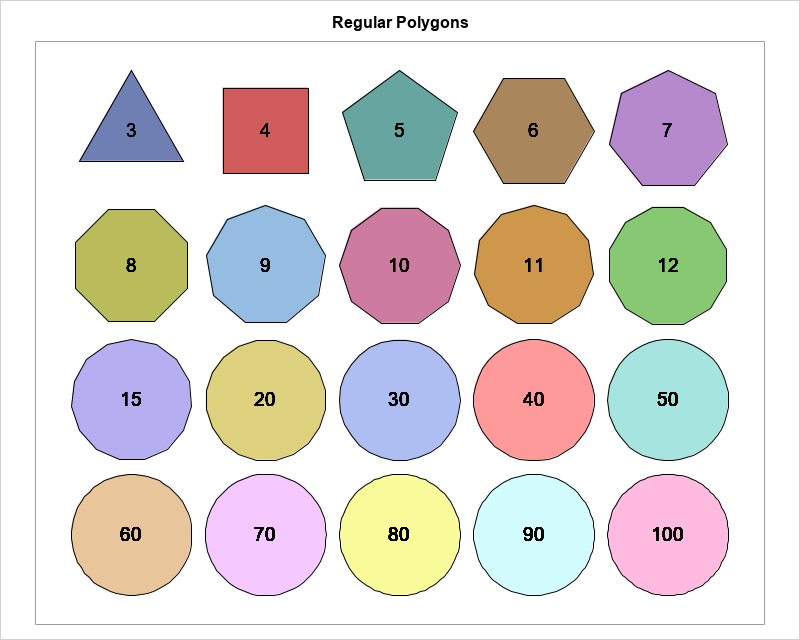
Recently, I saw a graphic on Twitter by @neilrkaye that showed the rapid convergence of a regular polygon to a circle as you increase the number of sides for the polygon. The author remarked that polygons that have 40 or more sides "all look like circles to me." That is, a regular polygon with a large number of sides is visually indistinguishable from a circle.

I had two reactions to the graphic. The first was "Cool! I want to create a similar figure in SAS!" (I have done so on the right; click to enlarge.) The second reaction was that the idea is both mathematically trivial and mathematically sophisticated. It is trivial because it is known to Archimedes more than 2,000 years ago and is readily understood by using high school math. But it is sophisticated because it is a particular instance of a mathematical limit, which is the foundation of calculus and the mathematical field of analysis.

The figure also demonstrates the fact that you can approximate a smooth object (a circle, a curve, a surface, ...) by a large number of small, local, linear approximations. It is not an exaggeration to say that that concept is among the most important concepts in applied mathematics. It is used in numerical methods to solve nonlinear equations, integrals, differential equations, and more. It is used in numerical optimization. It forms the foundations of computer graphics. A standard technique in computational algorithms that involves a nonlinear function is to approximate the function by the first term of the Taylor expansion—a process known as linearization.

An approximation of pi

Archimedes used this process (local approximation by a linear function) to approximate pi (π), which is the ratio of the circumference of a circle to its diameter. He used two sets of regular polygons: one that is inscribed in the unit circle and the other that circumscribes the unit circle. The circumference of an inscribed polygon is less than the circumference of the circle. The circumference of a circumscribed polygon is greater than the circumference of the circle. They converge to a common value, which is the circumference of the circle. If you apply this process to a unit circle, you approximate the value 2π. Archimedes used the same construction to approximate the area of the unit circle, which is π.

You can use Archimedes's ideas to approximate π by using trigonometry and regular polygons, as shown in the following paragraph.

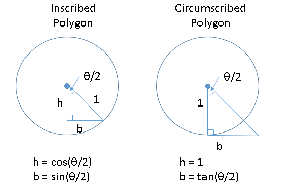
Suppose that a regular polygon has n sides. Then the central angle between adjacent vertices is θ = 2π/n radians. The following diagram illustrates the geometry of inscribed and circumscribed polygons. The right triangle that is shown is half of the triangle between adjacent vertices. Consequently,

• The half-length of a side is b, where b = sin(θ/2) for the inscribed polygon and b = tan(θ/2) for the circumscribed polygon.
• The height of the triangle is h, where h = cos(θ/2) for the inscribed polygon and h = 1 for the circumscribed polygon.
• The circumference of the regular polygon is 2 n b
• The area of the regular polygon is 2 n ( b h/2 ).

Approximate pi by using Archimedes's method

Although Archimedes did not have access to a modern computer, you can easily write a SAS DATA step program to reproduce Archimedes's approximations to the circumference and area of the unit circle, as shown below:

/* area and circomference */
data ApproxCircle;
pi = constant('pi');           /* Hah! We must know pi in order to evaluate the trig functions! */
do n = 3 to 100;
   angle = 2*pi/n;
   /* Circumference and Area for circumscribed polygon */
   b = tan(angle/2);
   h = 1;
   C_Out = 2*n * b;
   A_Out = 2*n * 0.5*b*h;
   /* Circumference and Area for inscribed polygon */
   b = sin(angle/2);
   h = cos(angle/2);
   C_In = 2*n * b;
   A_In = 2*n * 0.5*b*h;
   /* difference between the circumscribed and inscribed circles */
   CDiff = C_Out - C_In;
   ADiff = A_Out - A_In;
   output;
end;
label CDiff="Circumference Difference" ADiff="Area Difference";
keep n C_In C_Out A_In A_Out CDiff ADiff;
run;
 
/* graph the circumference and area of the n-gons as a function of n */
ods graphics / reset height=300px width=640px;
%let curveoptions = curvelabel curvelabelpos=min;
title "Circumference of Regular Polygons";
proc sgplot data=ApproxCircle;
   series x=n y=C_Out / &curveoptions;
   series x=n y=C_In  / &curveoptions;
   refline 6.2831853 / axis=y;              /* reference line at 2 pi */
   xaxis grid values=(0 to 100 by 10) valueshint;
   yaxis values=(2 to 10) valueshint label="Regular Polygon Approximation";
run;
 
title "Area of Regular Polygons";
proc sgplot data=ApproxCircle;
   series x=n y=A_Out / &curveoptions;
   series x=n y=A_In  / &curveoptions;
   refline 3.1415927 / axis=y;              /* reference line at pi */
   xaxis grid values=(0 to 100 by 10) valueshint;
   yaxis  values=(2 to 10) valueshint label="Regular Polygon Approximation";
run;

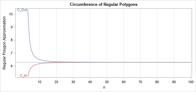
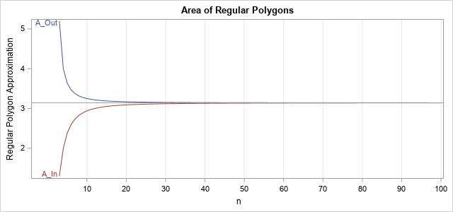
As you can see from the graph, the circumference and area of the regular polygons converge quickly to 2π and π, respectively. After n = 40 sides, the curves are visually indistinguishable from their limits, which is the same result that we noticed visually when looking at the grid of regular polygons.

The DATA step also computes the difference between the measurements of the circumscribed and inscribed polygons. You can print out a few of the differences to determine how close these estimates are to the circumference and area of the unit circle:

 
proc print data=ApproxCircle noobs;
   where n in (40, 50, 56, 60, 80, 100);
   var n CDiff ADiff;
run;

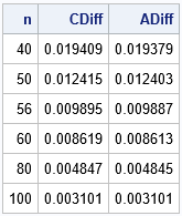
The table shows that the difference between the circumference of the circumscribed and inscribed polygons is about 0.02 when n = 40. For n = 56, the difference is less than 0.01, which means that the circumference of a regular polynomial approximates the circumference of the unit circle to two decimal places when n ≥ 56. If you use a regular 100-gon, the circumference is within 0.003 of the circumference of the unit circle. Although it is not shown, it turns out you need to use 177 sides before the difference is within 0.001, meaning that a 177-gon approximates the circumference of the unit circle to three decimal places.

Similar results hold for the area of the polygons and the area of a unit circle.

In conclusion, not only does a regular n-gon look very similar to the circle when n is large, but you can quantify how quickly the circumference and areas of an n-gon converges to the values 2 π and π, respectively. For n=56, the polygon values are accurate to two decimal places; for n=177, the polygon values are accurate to three decimal places.

Approximating a smooth curve by a series of discrete approximations is the foundation of calculus and modern numerical methods. The idea had its start in ancient Greece, but the world had to wait for Newton, Leibnitz, and others to provide the mathematical machinery (limits, convergence, ...) to understand the concepts rigorously.