Books about statistics and machine learning often discuss the tradeoff between bias and variance for an estimator. These discussions are often motivated by a sophisticated predictive model such as a regression or a decision tree. But the basic idea can be seen in much simpler situations. This article presents a simple situation that is discussed in a short paper by Dan Jeske (1993). Namely, if a random process produces integers with a known set of probabilities, what method should you use to predict future values of the process?

I will start by briefly summarizing Jeske's result, which uses probability theory to derive the best biased and unbiased estimators. I then present a SAS program that simulates the problem and compares two estimators, one biased and one unbiased.

A random process that produces integers

Suppose a gambler asks you to predict the next roll of a six-sided die. He will reward you based on how close your guess is to the actual value he rolls. No matter what number you pick, you only have a 1/6 chance of being correct. But if the strategy is to be close to the value rolled, you can compute the expected value of the six faces, which is 3.5. Assuming that the gambler doesn't let you guess 3.5 (which is not a valid outcome), one good strategy is to round the expected value to the nearest integer. For dice, that means you would guess ROUND(3.5) = 4. Another good strategy is to randomly guess either 3 or 4 with equal probability.

Jeske's paper generalizes this problem. Suppose a random process produces the integers 1, 2, ..., N, with probabilities p1, p2, ..., pN, where the sum of the probabilities is 1. (This distribution is sometimes called the "table distribution.") If your goal is to minimize the mean squared error (MSE) between your guess and a series of future random values, Jeske shows that the optimal solution is to guess the value that is closest to the expected value of the random variable. I call this method the ROUNDING estimator. In general, this method is biased, but it has the smallest expected MSE. Recall that the MSE is a measure of the quality of an estimator (smaller is better).

An alternative method is to randomly guess either of the two integers that are closest to the expected value, giving extra weight to the integer that is closer to the expected value. I call this method the RANDOM estimator. The random estimator is unbiased, but it has a higher MSE.

An example

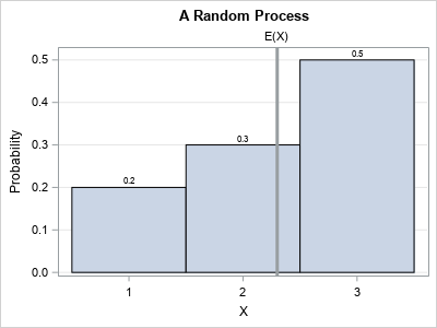
The following example is from Jeske's paper. A discrete process generates a random variable, X, which can take the values 1, 2, and 3 according to the following probabilities:

• P(X=1) = 0.2, which means that the value 1 appears with probability 0.2.
• P(X=2) = 0.3, which means that the value 2 appears with probability 0.3.
• P(X=3) = 0.5, which means that the value 3 appears with probability 0.5.

A graph of the probabilities is shown to the right. The expected value of this random variable is E(X) = 1(0.2) + 2(0.3) + 3(0.5) = 2.3. However, your guess must be one of the feasible values of X, so you can't guess 2.3. The best prediction (in the MSE sense) is to round the expected value. Since ROUND(2.3) is 2, the best guess for this example is 2.

Recall that an estimator for X is biased if its expected value is different from the expected value of X. Since E(X) ≠ 2, the rounding estimator is biased.

You can construct an unbiased estimator by randomly choosing the values 2 and 3, which are the two closest integers to E(X). Because E(X) = 2.3 is closer to 2 than to 3, you want to choose 2 more often than 3. You can make sure that the guesses average to 2.3 by guessing 2 with probability 0.7 and guessing 3 with probability 0.3. Then the weighted average of the guesses is 2(0.7) + 3(0.3) = 2.3, and this method produces an unbiased estimate. The random estimator is unbiased, but it will have a larger MSE.

Simulate the prediction of a random integer

Jeske proves these facts for an arbitrary table distribution, but let's use SAS to simulate the problem for the previous example. The first step is to compute the expected values of X. This is done by the following DATA step, which puts the expected value into a macro variable named MEAN:

/* Compute the expected value of X where 
   P(X=1) = 0.2
   P(X=2) = 0.3
   P(X=3) = 0.5
*/
data _null_;
array prob[3] _temporary_ (0.2, 0.3, 0.5);
do i = 1 to dim(prob);
   ExpectedValue + i*prob[i];       /* Sum of i*prob[i] */
end;
call symputx("Mean", ExpectedValue);
run;
 
%put &=Mean;

MEAN=2.3

The next step is to predict future values of X. For the rounding estimator, the predicted value is always 2. For the random estimator, let k be the greatest integer less than E(X) and let F = E(X) - k be the fractional part of E(x). To get an unbiased estimator, you can randomly choose k with probability 1-F and randomly choose k+1 with probability F. This is done in the following DATA step, which makes the predictions, generates a realization of X, and computes the residual difference for each method for 1,000 random values of X:

/* If you know mean=E(X)=expected value of X, Jeske (1993) shows that round(mean) is the best 
   MSE predictor, but it is biased.
   Randomly guessing the two closest integers is the best UNBIASED MSE predictor
   https://www.academia.edu/15728006/Predicting_the_value_of_an_integer-valued_random_variable
 
   Use these two predictors for 1000 future random variates.
*/
%let NumGuesses = 1000;
data Guess(keep = x PredRound diffRound PredRand diffRand);
call streaminit(12345);
array prob[3] _temporary_ (0.2, 0.3, 0.5);  /* P(X=i) */
 
/* z = floor(z) + frac(z) where frac(z) >= 0 */
/* https://blogs.sas.com/content/iml/2020/02/10/fractional-part-of-a-number-sas.html */
k = floor(&Mean);
Frac = &Mean - k;                        /* distance from E(X) to x */
do i = 1 to &NumGuesses;
   PredRound = round(&Mean);             /* guess the nearest integer */
   PredRand = k + rand("Bern", Frac);    /* random guesses between k and k+1, weighted by Frac */
   /* The guesses are made. Now generate a new instance of X and compute residual difference */
   x = rand("Table", of prob[*]);
   diffRound = x - PredRound;            /* rounding estimate */
   diffRand  = x - PredRand;             /* unbiased estimate */
   output;
end;
run;
 
/* sure enough, ROUND is the best predictor in the MSE sense */
proc means data=Guess n USS mean;
   var diffRound DiffRand;
run;

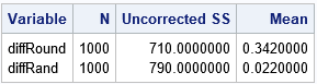
The output from PROC MEANS shows the results of generating 1,000 random integers from X. The uncorrected sum of squares (USS) column shows the sum of the squared residuals for each estimator. (The MSE estimate is USS / 1000 for these data.) The table shows that the USS (and MSE) for the rounding estimator is smaller than for the random estimator. On the other hand, The mean of the residuals is not close to zero for the rounding method because it is a biased method. In contrast, the mean of the residuals for the random method, which is unbiased, is close to zero.

It might be easier to see the bias of the estimators if you look at the predicted values themselves, rather than at the residuals. The following call to PROC MEANS computes the sample mean for X and the two methods of predicting X:

/* the rounding method is biased; the random guess is unbiased */
proc means data=Guess n mean stddev;
   var x PredRound PredRand;
run;

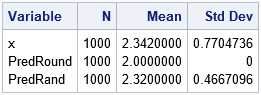
This output shows that the simulated values of X have a sample mean of 2.34, which is close to the expected value. In contrast, the rounding method always predicts 2, so the sample mean for that column is exactly 2.0. The sample mean for the unbiased random method is 2.32, which is close to the expected value.

In summary, you can use SAS to simulate a simple example that compares two methods of predicting the value of a discrete random process. One method is biased but has the lowest MSE. The other is unbiased but has a larger MSE. In statistics and machine learning, practitioners often choose between an unbiased method (such as ordinary least squares regression) and a biased method (such as ridge regression or LASSO regression). The example in this article provides a very simple situation that you can use to think about these issues.