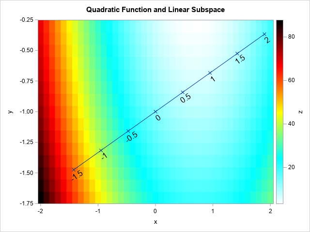
This article discusses how to restrict a multivariate function to a linear subspace. This is a useful technique in many situations, including visualizing an objective function that is constrained by linear equalities. For example, the graph to the right is from a previous article about how to evaluate quadratic polynomials. The graph shows a heat map for a quadratic polynomial of two variables. The diagonal line represents a linear constraint between the X and Y variables. If you restrict the polynomial to the diagonal line, you obtain a one-dimensional function that you can easily graph and visualize. By repeating this process for other lines, you can construct a "stack" of lower-dimensional slices that enable you to understand the graph of the original bivariate function.

This example generalizes. For a function of many variables, you can restrict the function to a lower-dimensional subspace. By visualizing the restricted function, you can understand the high-dimensional function better. I previously demonstrated this technique for multidimensional regression models by using the SLICEFIT option in the EFFECTPLOT statement in SAS. This article shows how to use ideas from vector calculus to restrict a function to a parameterized linear subspace.

Visualize high-dimensional data and functions

There are basically two techniques for visualizing high-dimensional objects: projection and slicing. Many methods in multivariate statistics compute a linear subspace such that the projection of the data onto the subspace has a desirable property. One example is principal component analysis, which endeavors to find a low dimensional subspace that captures most of the variation in the data. Another example is linear discriminant analysis, which aims to find a linear subspace that maximally separates groups in the data. In both cases, the data are projected onto the computed subspaces to reveal characteristics of the data. There are also statistical methods that attempt to find nonlinear subspaces.

Whereas projection is used for data, slicing is often used to visualize the graphs of functions. In regression, you model a response variable as a function of the explanatory variables. Slicing the function along a linear subspace of the domain can reveal important characteristics about the function. That is the method used by the SLICEFIT option in the EFFECTPLOT statement, which enables you to visualize multidimensional regression models. The most common "slice" for a regression model is to specify constant values for all but one continuous variable in the model.

When visualizing an objective function that is constrained by a set of linear equalities, the idea is similar. The main difference is that the "slice" is usually determined by a general linear combination of variables.

Restrict a function to a one-dimensional subspace

A common exercise in multivariate calculus is to restrict a bivariate function to a line. (This is equivalent to a "slice" of the bivariate function.) Suppose that you choose a point, x0, and a unit vector, u, which represents the "direction". Then a parametric line through x0 in the direction of u is given by the vector expression v(t) = x0 + t u, where t is any real number. If you restrict a multivariate function to the image of v, you obtain a one-dimensional function.

For example, consider the quadratic polynomial in two variables:
f(x,y) = (9*x##2 + x#y + 4*y##2) - 12*x - 4*y + 6
The function is visualized by the heat map at the top of this article. Suppose x0 = {0, -1} and choose u to be the unit vector in the direction of the vector {3, 1}. (This choice corresponds to a linear constraint of the form x – 3y = 3.)

The following SAS/IML program constructs the parameterized line v(t) for a uniform set of t values. The quadratic function is evaluated at this set of values and the resulting one-dimensional function is graphed:

proc iml;
/* Evaluate the quadratic function at each column of X and return a row vector. */
start Func(XY);
   x = XY[1,]; y = XY[2,];
   return (9*x##2  + x#y + 4*y##2) - 12*x - 4*y + 6;
finish;
 
x0 = {0, -1};          /* evaluate polynomial at this point */
d  = {3, 1};           /* vector that determines direction */
u  = d / norm(d);      /* unit vector (direction) */
 
t = do(-2, 2, 0.1);    /* parameter values */
v = x0 + t @ u;        /* evenly spaced points along the linear subspace */
f = Func(v);           /* evaluate the 2-D function along the 1-D subspace */
title "Quadratic Form Evaluated on Linear Subspace";
call series(t, f) grid={x y};

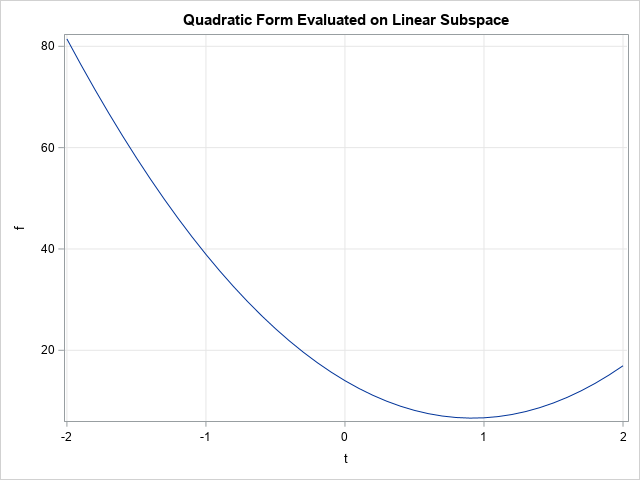
The graph shows the restriction of the 2-D function to the 1-D subspace. According to the graph, the restricted function reaches a minimum value for t ≈ 0.92. The corresponding (x, y) values and the corresponding function value are shown below:

tMin = 0.92;           /* t* = parameter near the minimum */
vMin = x0 + tMin * u;  /* corresponding (x(t*), y(t*)) */
fMin = Func(vMin);     /* f(x(t*), y(t*)) */
print tMin vMin fMin;

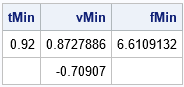
If you look back to the heat map at the top of this article, you will see that the value (x,y) = (0.87,-0.71) correspond to the location for which the function achieves a minimum value when restricted to the linear subspace. The value of the function at that (x,y) value is approximately 6.6.

The SAS/IML program uses the Kronecker direct-product operator (@) to create points along the line. The operation is v = x0 + t @ u. The symbols x0 and u are both column vectors with two elements. The Kronecker product creates a 2 x k matrix, where k is the number of elements in the row vector t. The Kronecker product enables you to vectorize the program instead of looping over the elements of t and forming the individual vectors x0 + t[i]*u.

You can generalize this example to evaluate a multivariate function on a two-dimensional subspace. If u1 and u2 are two orthogonal, p-dimensional, unit vectors, the expression x0 + s*u1 + t*u2 spans a two-dimensional subspace of R^p. You can use the ExpandGrid function in SAS/IML to generate ordered pairs (s, t) on a two-dimensional grid.

Summary

In summary, you can slice a multivariate function along a linear subspace. Usually, 1-D or 2-D subspaces are used and the resulting (restricted) function is graphed. This helps you to understand the function. You can choose a series of slices (often parallel to each other) and "stack" the slices in order to visualize the multivariate function. Typically, this technique works best for functions that have three or four continuous variables.

You can download the SAS program that creates the graphs in this article.