What is an efficient way to evaluate a multivariate quadratic polynomial in p variables? The answer is to use matrix computations! A multivariate quadratic polynomial can be written as the sum of a purely quadratic term (degree 2), a purely linear term (degree 1), and a constant term (degree 0). The purely quadratic term is called a quadratic form. This article shows how to use matrix computations to efficiently evaluate a multivariate quadratic polynomial.

Quadratic polynomials and matrix expressions

As I wrote in a previous article about optimizing a quadratic function, the matrix of second derivatives and the gradient of first derivatives appear in the matrix representation of a quadratic polynomial. I will use the same example as in my previous article. Namely, the following quadratic polynomial in two variables:
f(x,y) = (9*x##2 + x#y + 4*y##2) - 12*x - 4*y + 6
       = (1/2) x` Q x + L` x + 6
where Q = {18  1, 1  8} is a 2x2 symmetric matrix, L = {-12  -4} is a column vector, and x = {x, y} is a column vector that represents the coordinates at which to evaluate the quadratic function.

This example generalizes. Every quadratic function in p variables can be written as the sum of a quadratic form (1/2 x` Q x), a linear term (L` x) and a constant. Here Q is a p x p symmetric matrix of second derivatives (the Hessian matrix of f) and L and x are p-dimensional column vectors.

Evaluate quadratic polynomial in SAS

Because the computation involves vectors and matrices, the SAS/IML language is the natural place to use matrices to evaluate a quadratic function. The following SAS/IML statements implement a simple function to evaluate a quadratic polynomial (given in terms of Q, L, and a constant) at an arbitrary two-dimensional vector, x:

proc iml;
/* Evaluate  f(x) = 0.5 * x` * Q * x + L`*x + const, where
   Q is p x p symmetric matrix, 
   L and x are col vector with p elements.
   This version evaluates ONE vector x and returns a scalar value. */
start EvalQuad(x, Q, L, const=0);
   return 0.5 * x`*Q*x + L`*x + const;
finish;
 
/* compute Q and L for f(x,y)= 9*x##2 + x#y + 4*y##2) - 12*x - 4*y + 6 */
Q = {18 1,             /* matrix of second derivatives */
      1 8};
L = { -12, -4};        /* use column vectors for L and x */
const = 6;
x0 = {0, -1};          /* evaluate polynomial at this point */
f = EvalQuad(x0, Q, L, const);
print f[L="f(0,-1)"];

Evaluate a quadratic polynomial at multiple points

When I implement a function in the SAS/IML language, I try to "vectorize" it so that it can evaluate multiple points in a single call. Often you can use matrix operations to vectorize a function evaluation, but I don't see how to make the math work for this problem. The natural way to evaluate a quadratic polynomial at k vectors X1, X2, ..., Xk, is to pack those vectors into a p x k matrix X such that each column of X is a point at which to evaluate the polynomial. Unfortunately, the matrix computation of the quadratic form M = 0.5 * X`*Q*X results in a k x k matrix. Only the k diagonal elements are needed for evaluating the polynomial on the k input vectors, so although it is possible to compute M, doing so would be very inefficient.

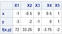
In this case, it seems more efficient to loop over the columns of X. The following function implements a SAS/IML module that evaluates a quadratic polynomial at every column of X and returns a row vector of the results. The module is demonstrated by calling it on a matrix that has 5 columns.

/* Evaluate the quadratic function at each column of X and return a row vector. */
start EvalQuadVec(X, Q, L, const=0);
   f = j(1, ncol(X), .);
   do i = 1 to ncol(X);
      v = X[,i];
      f[i] = 0.5 * v`*Q*v + L`*v + const;
   end;
   return f;
finish;
 
/*    X1  X2  X3 X4  X5  */
vx = {-1 -0.5 0  0.5 1 ,
      -3 -2  -1  0   1 };
f = EvalQuadVec(vx, Q, L, const=0);
print (vx // f)[r={'x' 'y' 'f(x,y)'} c=('X1':'X5')];

Evaluate a quadratic polynomial on a uniform grid of points

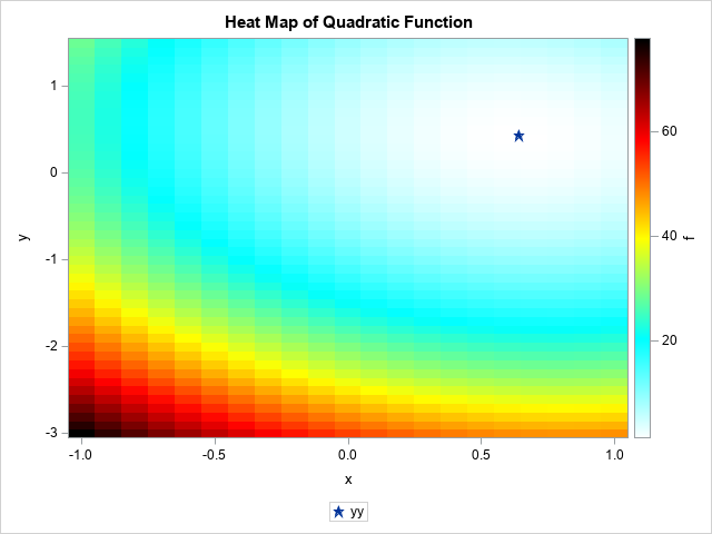
You can use the EvalQuadVec function to evaluate a quadratic polynomial on any set of multiple points. In particular, you can use the ExpandGrid function to construct a regular 2-D grid of points. By evaluating the function at each point on the grid, you can visualize the function. The following statements create a heat map of the function on a regular grid. The heat map is shown at the top of this article.

x = do(-1, 1, 0.1); 
y = do(-3, 1.5, 0.1);
xy = expandgrid(x, y);             /* 966 x 2 matrix */
f = EvalQuadVec(xy`, Q, L, const); /* evaluate polynomial at all points */
 
/* write results to a SAS data set and visualize the function by using a heat map */
M = xy || f`;
create Heatmap from M[c={'x' 'y' 'f'}];  append from M;  close;
QUIT;
 
data optimal;
   xx=0.64; yy=0.42;  /* optional: add the optimal (x,y) value */
run;
data All;  set Heatmap optimal; run;
 
title "Heat Map of Quadratic Function";
proc sgplot data=All;
   heatmapparm x=x y=y colorresponse=f / colormodel= (WHITE CYAN YELLOW RED BLACK);
   scatter x=xx y=yy / markerattrs=(symbol=StarFilled);
   xaxis offsetmin=0 offsetmax=0;
   yaxis offsetmin=0 offsetmax=0;
run;

Quadratic approximations

Perhaps you do not often use quadratic polynomials. This technique is useful even for general nonlinear functions because it enables you to find the best quadratic approximation to a multivariate function at any point x0. The multivariate Taylor series at the point x0, truncated at second order, is
f(x) ≈ f(x0) + L` · (x – x0) + (1/2) (x – x0)` · Q · (x – x0)
where L = ∇f(x0) is the gradient of f evaluate at x0 and Q = D²f(x0) is the symmetric Hessian matrix of second derivatives of f evaluated at x0.

Summary

In summary, you can use matrix computations to evaluate a multivariate quadratic polynomial. This article shows how to evaluate a quadratic polynomial at multiple points. For a polynomial of two variables, you can use this technique to visualize quadratic functions.

You can download the SAS program that creates the graphs in this article.