I frequently see questions on SAS discussion forums about how to compute the geometric mean and related quantities in SAS. Unfortunately, the answers to these questions are sometimes confusing or even wrong. In addition, some published papers and web sites that claim to show how to calculate the geometric mean in SAS contain wrong or misleading information.
This article shows how to compute the geometric mean, the geometric standard deviation, and the geometric coefficient of variation in SAS. It first shows how to use PROC TTEST to compute the geometric mean and the geometric coefficient of variation. It then shows how to compute several geometric statistics in the SAS/IML language. Lastly, the SAS file that accompanies this article contains a SAS/IML function (geoStats) that makes it easy to compute the statistics and their confidence intervals.
For an introduction to the geometric mean, see "What is a geometric mean." For information about the (arithmetic) coefficient of variation (CV) and its applications, see the article "What is the coefficient of variation?"
Compute the geometric mean and geometric CV in SAS
As discussed in my previous article, the geometric mean arises naturally when positive numbers are being multiplied and you want to find the average multiplier. Although the geometric mean can be used to estimate the "center" of any set of positive numbers, it is frequently used to estimate average values in a set of ratios or to compute an average growth rate.
The TTEST procedure is the easiest way to compute the geometric mean (GM) and geometric CV (GCV) of positive data. To demonstrate this, the following DATA step simulates 100 random observations from a lognormal distribution. PROC SGPLOT shows a histogram of the data and overlays a vertical line at the location of the geometric mean.
%let N = 100; data Have; call streaminit(12345); do i = 1 to &N; x = round( rand("LogNormal", 3, 0.8), 0.1); /* generate positive values */ output; end; run; title "Geometric Mean of Skewed Positive Data"; proc sgplot data=Have; histogram x / binwidth=10 binstart=5 showbins; refline 20.2 / axis=x label="Geometric/Mean" splitchar="/" labelloc=inside lineattrs=GraphData2(thickness=3); xaxis values=(0 to 140 by 10); yaxis offsetmax=0.1; run; |
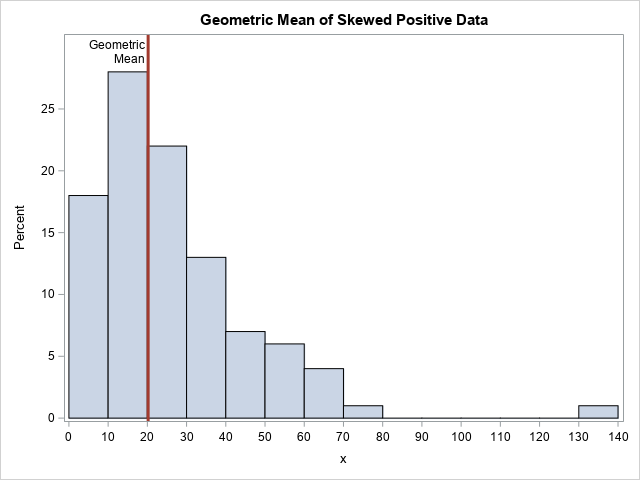
Where is the "center" of these data? That depends on your definition. The mode of this skewed distribution is close to x=15, but the arithmetic mean is about 26.4. The mean is pulled upwards by the long right tail. It is a mathematical fact that the geometric mean of data is always less than the arithmetic mean. For these data, the geometric mean is 20.2.
To compute the geometric mean and geometric CV, you can use the DIST=LOGNORMAL option on the PROC TTEST statement, as follows:
proc ttest data=Have dist=lognormal; var x; ods select ConfLimits; run; |
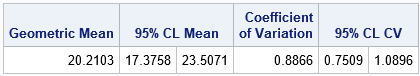
The geometric mean, which is 20.2 for these data, estimates the "center" of the data. Notice that the procedure does not report the geometric standard deviation (or variance), but instead reports the geometric coefficient of variation (GCV), which has the value 0.887 for this example. The documentation for the TTEST procedure explains why the GCV is the better measure of variation: "For lognormal data, the CV is the natural measure of variability (rather than the standard deviation) because the CV is invariant to multiplication of [the data]by a constant."
You might wonder whether data need to be lognormally distributed to use this table. The answer is that the data do not need to be lognormally distributed to use the geometric mean and geometric CV. However, the 95% confidence intervals for these quantities assume log-normality.
Definitions of geometric statistics
As T. Kirkwood points out in a letter to the editors of Biometric (Kirkwood, 1979), if data are lognormally distributed as LN(μ σ), then
- The quantity GM = exp(μ) is the geometric mean. It is estimated from a sample by the quantity exp(m), where m is the arithmetic mean of the log-transformed data.
- The quantity GSD = exp(σ) is defined to be the geometric standard deviation. The sample estimate is exp(s), where s is the standard deviation of the log-transformed data.
- The geometric standard error (GSE) is defined by exponentiating the standard error of the mean of the log-transformed data. Geometric confidence intervals are handled similarly.
- Kirkwood's proposal for the geometric coefficient of variation (GCV) is not generally used. Instead, the accepted definition of the GCV is GCV = sqrt(exp(σ2) – 1), which is the definition that is used in SAS. The estimate for the GCV is sqrt(exp(s2) – 1).
You can use these formulas to compute the geometric statistics for any positive data. However, only for lognormal data do the statistics have a solid theoretical basis: transform to normality, compute a statistic, apply the inverse transform.
Compute the geometric mean in SAS/IML
You can use the SAS/IML language to compute the geometric mean and other "geometric statistics" such as the geometric standard deviation and the geometric CV. The GEOMEAN function is a built-in SAS/IML function, but the other statistics are implemented by explicitly computing statistics of the log-transformed data, as described in the previous section:
proc iml; use Have; read all var "x"; close; /* read in positive data */ GM = geomean(x); /* built-in GEOMEAN function */ print GM; /* To estimate the geometric mean and geometric StdDev, compute arithmetic estimates of log(X), then EXP transform the results. */ n = nrow(x); z = log(x); /* log-transformed data */ m = mean(z); /* arithmetic mean of log(X) */ s = std(z); /* arithmetic std dev of log(X) */ GM2 = exp(m); /* same answer as GEOMEAN function */ GSD = exp(s); /* geometric std dev */ GCV = sqrt(exp(s**2) - 1); /* geometric CV */ print GM2 GSD GCV; |
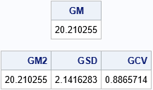
Note that the GM and GCV match the output from PROC TTEST.
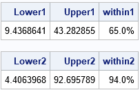
What does the geometric standard deviation mean? As for the arithmetic mean, you need to start by thinking about the location of the geometric mean (20.2). If the data are normally distributed, then about 68% of the data are within one standard deviation of the mean, which is the interval [m-s, m+s]. For lognormal data, about 68% of the data should be in the interval [GM/GSD, GM*GSD] and, in fact, 65 out of 100 of the simulated observations are in that interval. Similarly, about 95% of lognormal data should be in the interval [GM/GSD2, GM*GSD2]. For the simulated data, 94 out of 100 observations are in the interval, as shown below:
I am not aware of a similar interpretation of the geometric coefficient of variation. The GCV is usually used to compare two samples. As opposed to the confidence intervals in the previous paragraph, the GCV does not make any reference to the geometric mean of the data.
Other ways to compute the geometric mean
The methods in this article are the simplest ways to compute the geometric mean in SAS, but there are other ways.
- You can use the DATA step to log-transform the data, use PROC MEANS to compute the descriptive statistics of the log-transformed data, then use the DATA step to exponentiate the results.
- You can use the OUTTABLE= option in PROC UNIVARIATE, which creates a SAS data set that contains many univariate statistics, including the geometric mean.
- PROC SURVEYMEANS can compute the geometric mean (with confidence intervals) and the standard error of the geometric mean for survey responses. However, the variance of survey data is not the same as the variance of a random sample, so you should not use the standard error statistic unless you have survey data.
As I said earlier, there is some bad information out there on the internet about this topic, so beware. A site that seems to get all the formulas correct and present the information in a reasonable way is Alex Kritchevsky's blog.
You can download the complete SAS program that I used to compute the GM, GSD, and GCV. The program also shows how to compute confidence intervals for these quantities. Finally, the program includes a SAS/IML function, geoStats, that makes it easy to compute the geometric statistics in SAS.
WANT MORE GREAT INSIGHTS MONTHLY? | SUBSCRIBE TO THE SAS TECH REPORT

25 Comments
SAS IT Resource Management provides support for geometric and weighted geometric means. I'm not sure how much it is used in practice by customers.
Is it a spoiler alert to suggest you'll be blogging about harmonic mean in the future? (and is it possible to talk about harmonic means without referencing trains from Chicago and New York?)
Very good post!
Thanks for writing. No, I wasn't planning to write about the harmonic mean (the third of the classical means that were known to Pythagoras). I haven't seen many questions about that topic from SAS users. But if I ever write about it, I will endeavor to avoid trains.
PROC UNIVARIATE can output GEOMEAN directly, but not GSD and GCV.
Thanks. As far as I know, you can request that UNIVARIATE create an output data set that contains the geometric mean. You can also put it in an inset for a graph. But I don't think it appears in any tables.
Rick,
which is the interval [m0s, m+s]
should be
which is the interval [m-s, m+s]
?
Yes. Thank you for finding that typo. I have fixed it.
Could be that you need to take care of the special case of any 0 derivating in data step? I saw that you keep only positive, but geometric mean of a subset with a 0 is 0, sice by definition is the root of a product.
Thanks for writing. Yes, in the mathematical definition of the geometric mean (the nth root of a product), a single zero will cause the geometric mean itself to be zero. In statistics, the data must be strictly positive. When the data are positive, an equivalent definition is the mean of the logged values: (1/n) Sum of log(x_i).
The issue of zero (or even negative) values is a big mess. There have been several papers on the topic, but none of the techniques are widely accepted.
In practice, measurements have a lower limit based on the precision of the measuring instrument. For example, if a scientist is measuring lead in drinking water, the standard test has a detection limit of perhaps 0.05 μg/L. If a sample measures "zero", it really means that the amount of lead is below the threshold. The EPA has various guidelines (I am not an expert on them) that tell researchers how to report these numbers. For example, you could report the threshold (0.05) or half the threshold (0.025) or 0. But as you point out, if you record 0 then the entire (mathematical) answer is zero, which tells you nothing about the values of the other samples. If you use 0.025 versus 0.05, you get very different answers. The lesson is that the geometric mean is very sensitive to data values that are close to zero.
Rick, Nice article , It helped me to understand the concepts. Is there any new way of Computing the geometric mean, geometric standard deviation, and geometric CV? I wanted to know what are the alternative solutions available. And i was trying to do the same using python libraries , if you know corresponding python solutions , then please suggest.
Can geometric mean be reported as 20.2 (9.44 - 43.3)? I'm not sure if this is an acceptable notation and I can't really find examples of this but it makes sense so I want to know if it is typically done that way? Most are not familiar with the */ notation and it might just be easier to understand the "range" notation.
Many fields report a statistic and CI as you describe. When I wrote "95% of lognormal data should be in the interval [GM/GSD^2, GM*GSD^2]" I did not intend for anyone to write it like that. Plug in the numbers and report the interval.
Thanks for the nice article. The documentation for the TTEST procedure says: "For lognormal data, the CV is the natural measure of variability (rather than the standard deviation) because the CV is invariant to multiplication of [the data]by a constant." Is this explanation suffficient to support that GCV is better? According to math derivation, the GSD is also invariant to multiplication of the original data by a constant, and this can be verified in the code of example:
proc iml;
use Have; read all var "x"; close;
GM = geomean(10*x); /* 10 times orignal data */
print GM;
n = nrow(x);
z = log(10*x); /* 10 times orignal data */
m = mean(z);
s = std(z);
GM2 = exp(m);
GSD = exp(s); /* geometric std dev is invariant*/
GCV = sqrt(exp(s**2) - 1); /* geometric CV is invariant*/
print GM2 GSD GCV;
quit;
You are correct. As to why the CV is preferred, it could be a convention, but it could also be that the CV for the lognormal distribution is invariant under changes of the mean where the SD is not:
Great post! I am trying to obtain geometric mean ratio and its 95% confidence interval (CI) as well.
I tried obtaining using proc ttest as well as proc genmod (done after applying natural log to the data) but noticed that the 95% CI is slightly different. Which should I use?
Here my codes:
proc ttest data=im_s dist=lognormal;
var as;
class trt;
by vis;
run;
proc genmod data=im_s;
class trt vis;
model ln_as = trt*vis;
lsmeans trt*vis / diff exp cl;
run;
I think you should post this question and sample data to the SAS Support Communities if you want a thorough discussion. Briefly, these are different (but related) models, so you shouldn't expect the same answers. The second model incorporates VIS into the model, so if you want to make comparisons at different levels of VIZ, you might want to use that model. A third model is:
model as = trt*vis / link=log;
Two relevant articles:
- "The difference between CLASS statements and BY statements in SAS," which show how the models are related.
- "Error distributions and exponential regression models," which compares your GENMOD model and the one with LINK=LOG.
Hello Rick I am interesting in using this GSD as a denominator in Geometric Sharpe Ratio to compare risk adjusted returns of various investments. I am wondering considering stock returns show fat tails and skewness even for log returns is the GSD still suitable to measure risk? I know Traditional S.D. does not require Gaussian Distribution in order to be used as a way to compare relative risk of different investments so I am wondering whether this is also true for GSD.
Thanks.
> is GSD still suitable to measure risk?
I don't think I can answer whether the geometric SD is suitable for your application. However, what you say is true. Just as the SD is used as a general measure of scale for non-Gaussian distributions, the GSD is a measure of scale for distributions that have properties (semi-bounded) that are similar to the lognormal.
Thanks Rick for replying to my comment! I want to ask are stock and gold returns distribution semi bounded considering there are negative returns?
I am not an expert in the distribution of stock and gold returns. I suggest you ask a financial modeler.
Mathematically, the distribution of returns when you "buy long" is semi-bounded. It is bounded below because the most you can lose is 100%. It is not bounded above because the share price has no upper limit.
If you hope to use the geometric distribution, you cannot use the returns because they can be negative. Convert the returns into proportions, which are always positive. For example, an annual return of -10% means that the new value of your investment is now 0.9 the value from the previous year.
Thanks again for replying Rick! So I guess this means I can use Geo S.D. as a way to compare risk of different investments just like Traditional S.D. What I do to calculate Geo SD is first I compute the log returns by adding every return by 1 to make sure the returns are positive and then take natural logarithm of the number. I found though the natural logarthim can be either negative or positive even though I add 1 to every return. Then I take the standard deviation of these log returns and I get the SD by taking the exponent of the standard deviation of log returns and subtracting 1. I hope this isn't wrong.
Thanks.
Sorry for asking too much questions but I am wondering the semi bounded distribution can also be for assets which are having high negative skew? Like Selling Call Options. The Loss is Infinity while the Gain is Limited to the Premium Recieved from selling the options. When I looked up semi bounded distribnutions all the examples were for distributions that value cannot go below 0 but has no limit on upper bound hence the question.
Thanks.
You would be wise to seek advice from someone who is an expert in the modeling of investments.
To recompute the 95% CL Mean from the example:
17.37585 ; 23.50713
/* to find the tCrit here -> 1.984217*/
proc iml;
alpha = 0.05;
n=100;
tCrit = quantile("T", 1 - alpha/2, n-1);
print(tCrit);
quit;
geomean / exp(tCrit * SEM)
geomean * exp(tCrit * SEM)
95% CL Mean from the example:
17.37585 =
20.2103 / exp( 1.984217 * log(2.1416283)/10 )
23.50713 =
20.2103 * exp( 1.984217 * log(2.1416283)/10 )
Hi Rick
The CV for a lognormal random variable is sqrt(exp(σ^2) – 1). Using the DIST=LOGNORMAL option on the PROC TTEST statement estimates this CV by sqrt(exp(s^2) – 1) rather than the usual sample CV. I notice that nowhere in the PROC TTEST documentation is the term GCV used - and rightly so in my opinion.
Kirkwood's definition of GCV = 100(GSD-1)% seems to be used to describe inter-laboratory and intra-laboratory variation in assay results in a number of academic publications.
Unlike the CV, Kirkwood's GCV was an attempt to describe variation about the geometric mean. He viewed it as an alternative to reporting the GSD. Instead of GSD = 2.14, GCV = 114% expresses how much to increase the GM by to get GM*GSD. Though searching for the phrases "geometric standard deviation" and "geometric coefficient of variation" on Google Scholar makes me think the GSD is a much more popular term than the GCV.
I am curious why you think "Kirkwood's GCV is not generally used. Instead, the accepted definition of the GCV is GCV = sqrt(exp(σ^2) – 1)”?
Thanks for writing. This article is from years ago, but I think the issue is that Kirkwood's statistic is not an estimate of the CV for a log-normal distribution. Kirkwood proposed his statistic in a short letter to the editor as a way to communicate the meaning of the log-normal scale to "non-statisticians" and to "those who have little facility with numbers" (Kirkwood, 1979, p. 908-909) who are familiar with arithmetic means and deviations. If Kirkwood's statistic helps you to communicate the dispersion in data, that's awesome.