An important application of the dot product (inner product) of two vectors is to determine the angle between the vectors. If u and v are two vectors, then
cos(θ) = (u ⋅ v) / (|u| |v|)
You could apply the inverse cosine function if you wanted to find θ in [0, π], but since the cosine function is a monotonic decreasing transformation on [0, π], it is usually sufficient to know the cosine of the angle between two vectors. The expression (u ⋅ v) / (|u| |v|) is called the cosine similarity between the vectors u and v. It is a value in [-1, 1]. This article discusses the cosine similarity, why it is useful, and how you can compute it in SAS.

What is the cosine similarity?

For multivariate numeric data, you can compute the cosine similarity of the rows or of the columns. The cosine similarity of the rows tells you which subjects are similar to each other. The cosine similarity of the columns tells you which variables are similar to each other. For example, if you have clinical data, the rows might represent patients and the variables might represent measurements such as blood pressure, cholesterol, body-mass index, and so forth. The row similarity compares patients to each other; the column similarity compares vectors of measurements.

Vectors that are very similar to each other have a cosine similarity that is close to 1. Vectors that are nearly orthogonal have a cosine similarity near 0. Vectors that point in opposite directions have a cosine similarity of –1. However, in practice, the cosine similarity is often used on vectors that have nonnegative values. For those vectors, the angle between them is never more than 90 degrees and so the cosine similarity is between 0 and 1.

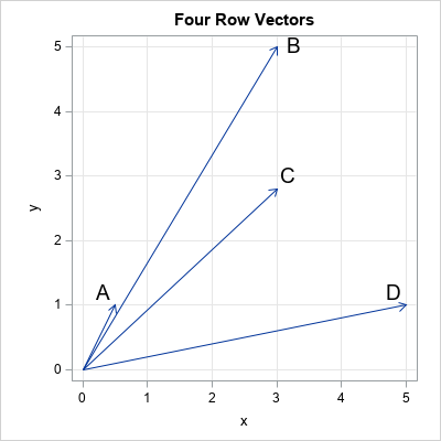
To illustrate how to compute the cosine similarity in SAS, the following statements create a simple data set that has four observations and two variables. The four row vectors are plotted:

data Vectors;
length Name $1;
input Name x y;
datalines;
A  0.5 1
B  3   5
C  3   2.8
D  5   1
;
 
ods graphics / width=400px height=400px;
title "Four Row Vectors";
proc sgplot data=Vectors aspect=1;
   vector x=x y=y / datalabel=Name datalabelattrs=(size=14);
   xaxis grid;  yaxis grid;
run;

The cosine similarity of observations

If you look at the previous graph of vectors and think that vector A is unlike the other vectors, then you are using the magnitude (length) of the vectors to form that opinion. The cosine similarity does not use the magnitude of the vectors to decide which vectors are alike. Instead, it uses only the direction of the vectors. You can visualize the cosine similarity by plotting the normalized vectors that have unit length, as shown in the next graph.

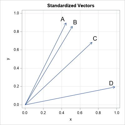
The second graph shows the vectors that are used to compute the cosine similarity. For these vectors, A and B are most similar to each other. Vector C is more similar to B than to D, and D is least similar to the others. You can use PROC DISTANCE and the METHOD=COSINE option to compute the cosine similarity between observations. If your data set has N observations, the result of PROC DISTANCE is an N x N matrix of cosine similarity values. The (i,j)th value is the similarity between the i_th vector and the j_th vector.

proc distance data=Vectors out=Cos method=COSINE shape=square;
   var ratio(_NUMERIC_);
   id Name;
run;
proc print data=Cos noobs; run;

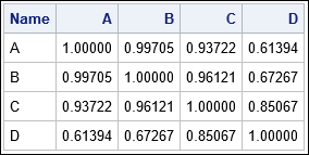
The results of the DISTANCE procedure confirm what we already knew from the geometry. Namely, A and B are most similar to each other (cosine similarity of 0.997), C is more similar to B (0.937) than to D (0.85), and D is not very similar to the other vectors (similarities range from 0.61 to 0.85).

Notice that the cosine similarity is not a linear function of the angle between vectors. The angle between vectors B and A is 4 degrees, which has a cosine of 0.997. The angle between vectors B and C is almost four times as big (16 degrees) but the cosine similarity is 0.961, which is not very different from 0.997 (and certainly not four times as small). Notice also that the graph of the cosine function is flat near θ=0. Consequently, the cosine similarity does not vary much between the vectors in this example.

Compute cosine similarity in SAS/IML

SAS/STAT does not include a procedure that computes the cosine similarity of variables, but you can use the SAS/IML language to compute both row and column similarity. The following PROC IML statements define functions that compute the cosine similarity for rows and for columns. To support missing values in the data, the functions use listwise deletion to remove any rows that contain a missing value. All functions are saved for future use.

/* Compute cosine similarity matrices in SAS/IML */
proc iml;
/* exclude any row with a missing value */
start ExtractCompleteCases(X);
   if all(X ^= .) then return X;
   idx = loc(countmiss(X, "row")=0);
   if ncol(idx)>0 then return( X[idx, ] );
   else                return( {} ); 
finish;
 
/* compute the cosine similarity of columns (variables) */
start CosSimCols(X, checkForMissing=1);
   if checkForMissing then do;    /* by default, check for missing and exclude */
      Z = ExtractCompleteCases(X);
      Y = Z / sqrt(Z[##,]);       /* stdize each column */
   end;
      else Y = X / sqrt(X[##,]);  /* skip the check if you know all values are valid */
   cosY = Y` * Y;                 /* pairwise inner products */
   /* because of finite precision, elements could be 1+eps or -1-eps */
   idx = loc(cosY> 1); if ncol(idx)>0 then cosY[idx]= 1; 
   idx = loc(cosY<-1); if ncol(idx)>0 then cosY[idx]=-1; 
   return cosY;
finish;
 
/* compute the cosine similarity of rows (observations) */
start CosSimRows(X);
   Z = ExtractCompleteCases(X);  /* check for missing and exclude */
   return T(CosSimCols(Z`, 0));  /* transpose and call CosSimCols */
finish;
store module=(ExtractCompleteCases CosSimCols CosSimRows);

Visualize the cosine similarity matrix

When you compare k vectors, the cosine similarity matrix is k x k. When k is larger than 5, you probably want to visualize the similarity matrix by using heat maps. The following DATA step extracts two subsets of vehicles from the Sashelp.Cars data set. The first subset contains vehicles that have weak engines (low horsepower) whereas the second subset contains vehicles that have powerful engines (high horsepower). You can use a heat map to visualize the cosine similarity matrix between these vehicles:

data Vehicles;
   set sashelp.cars(where=(Origin='USA'));
   if Horsepower < 140 OR Horsepower >= 310;
run;
proc sort data=Vehicles; by Type; run;  /* sort obs by vehicle type */
 
ods graphics / reset;
proc iml;
load module=(CosSimCols CosSimRows);
use Vehicles;
read all var _NUM_ into X[c=varNames r=Model]; 
read all var {Model Type}; close;
 
labl = compress(Type + ":" + substr(Model, 1, 10));
cosRY = CosSimRows(X);
call heatmapcont(cosRY) xvalues=labl yvalues=labl title="Cosine Similarity between Vehicles";

The heat map shows the cosine similarities of the attributes of 20 vehicles. Vehicles of a specific type (SUV, sedan, sports car,...) tend to be similar to each other and different from vehicles of other types. The four sports cars stand out. They are very dissimilar to the sedans, and they are also dissimilar to the SUVs and wagons.

Notice the small range for the cosine similarity values. Even the most dissimilar vehicles have a cosine similarity of 0.99.

Cosine similarity of columns

You can treat each row data as a vector of dimension p. Similarly (no pun intended!), you can treat each column as a vector of length N. You can use the CosSimCols function, defined in the previous section, to compute the cosine similarity matrix of numerical columns. The math is the same but is applied to the transpose of the data matrix. To demonstrate the function, the following statements compute and visualize the column similarity for the Vehicles data. There are 10 numerical variables in the data.

cosCY = CosSimCols(X);
call heatmapcont(cosCY) xvalues=varNames yvalues=varNames title="Cosine of Angle Between Variables";

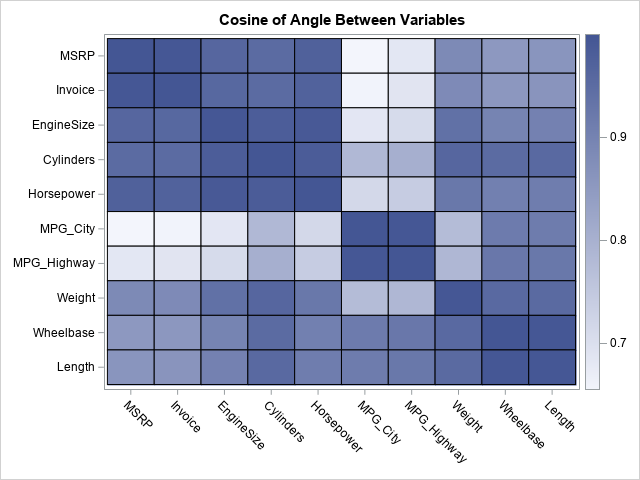
The heat map for the columns is shown. You can see that the MPG_City and MPG_Highway variables are dissimilar to most other variables, but similar to each other. Other sets of similar variables include the variables that measure cost (MSRP and Invoice), the variables that measure power (EngineSize, Cylinders, Horsepower), and the variables that measure size (Wheelbase, Length, Weight).

The connection between cosine similarity and correlation

The similarity matrix of the variables shows which variables are similar and dissimilar. In that sense, the matrix might remind you of a correlation matrix. However, there is an important difference: The correlation matrix displays the pairwise inner products of centered variables. The cosine similarity does not center the variables. Although the correlation is scale-invariant and affine invariant, the cosine similarity is not affine invariant: If you add or subtract a constant from a variable, its cosine similarity with other variables will change.

When the data represent positive quantities (as in the Vehicles data), the cosine similarity between two vectors can never be negative. For example, consider the relationship between the fuel economy variables (MPG_City and MPG_Highway) and the "power" and "size" variables. Intuitively, the fuel economy is negatively correlated with power and size (for example, Horsepower and Weight). However, the cosine similarity is positive, which shows another difference between correlation and cosine similarity.

Why is the cosine similarity useful?

The fact that the cosine similarity does not center the data is its biggest strength (and also its biggest weakness). The cosine similarity is most often used in applications in which the variables represent counts or indicator variables. Often, each row represents a document such as a recipe, a book, or a song. The columns indicate an attribute such as an ingredient, word, or musical technique.

For text documents, the number of columns (which represent important words) can be in the thousands. The goal is to discover which documents are structurally similar to each other, perhaps because they share similar content. Recommender engines can use the cosine similarity to suggest new books or articles that are similar to one that was previously read. The same technique can recommend similar recipes or similar songs.

The advantage of the cosine similarity is its speed and the fact that it is very useful for sparse data. In a future article, I'll provide a simple example that demonstrates how you can use the cosine similarity to find recipes that are similar or dissimilar to each other.

You can download the SAS program that computes the cosine similarities and creates the graphs in this article.