In response to a recent article about how to compute the cosine similarity of observations, a reader asked whether it is practical (or even possible) to perform these types of computations on data sets that have many thousands of observations. The problem is that the cosine similarity matrix is an N x N matrix, where N is the sample size. Thus, the matrix can be very big even for moderately sized data.

The same problem exists for all distance- and similarity-based measurements. Because the Euclidean distance is familiar to most readers, I will use distance to illustrate the techniques in this article. To be specific, suppose you have N=50,000 observations. The full distance matrix contains 2.5 billion distances between pairs of observations. However, in many applications, you are not interested in all the distances. Rather, you are interested in extreme distances, such as finding observations that are very close to each other or are very far from each other. For definiteness, suppose you want to find observations that are less than a certain distance from each other. That distance (called the cutoff distance) serves as a filter. Instead of storing N² observations, you only need to store the observations that satisfy the cutoff criterion.

Compute by using block-matrix computations

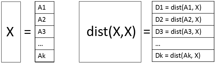
A way to perform a distance computation is to divide the data into blocks and perform block-matrix computations. If X is the data matrix, then the pairwise distance matrix of the N rows is an N x N matrix. But you can subdivide X into blocks where each block has approximately M rows, where M is a smaller number such as M=1,000. Write X = [A1, A2, ..., Ak], where the block matrices are stacked vertically. Then the full distance matrix D = dist(X, X) is equal to stacking the distance matrices for each of the block matrices: D = [dist(A1,X), dist(A2,X), ..., dist(Ak,X)]. Each of the block matrices is an M x N matrix. The following diagram shows the block-matrices. The main idea is to compute each block matrix (which fits into memory), then identify and extract the values that satisfy the cutoff distance. With this technique, you never hold the full N x N distance matrix in memory.

A small example of block computations

A programming principle that I strongly endorse is "start small." Even if your goal is to work with large data, develop and debug the program for small data. In this section, the data contains only 13 observations and 10 variables. The goal is to use block-matrix computations (with a block size of M=3) to compute the 13² = 169 pairwise distances between the observations. As each block of distances is computed, those distances that are less than 2 (the cutoff distance in this example) are identified and stored. The data are simulated by using the following DATA step:

/* start with a smaller example: 13 observations and 10 vars */
%let N = 13;
data Have;
call streaminit(12345);
array x[10];
do i = 1 to &N;
   do j = 1 to dim(x);   x[j] = rand("Uniform", -1, 1);  end;
   output;
end;
keep x:;
run;

It makes sense to report the results by giving the pair of observations numbers and the distance for those pairs that satisfy the criterion. For these simulated data, there are 10 pairs of observations that are closer than 2 units apart, as we shall see shortly.

The following SAS/IML program shows how to use block computation to compute the pairs of observations that are close to each other. For illustration, set the block size to M=3. Suppose you are computing the second block, which contains the observations 4, 5, and 6. The following program computes the distance matrix from those observations to every other observation:

proc iml;
use Have; read all var _NUM_ into X; close;
m = 3;                       /* block size */
n = nrow(X);                 /* number of observations */
cutoff = 2;                  /* report pairs where distance < cutoff */
 
/* Block matrix X = [A1, A2, A3, ..., Ak]  */
startrow=4; endrow=6;        /* Example: Look at 2nd block with obs 4,5,6 */
rows = startRow:endRow;
 
/* Compute D_i = distance(Ai, X)         */
A = X[rows,];               /* extract block */
D = distance(A, X);         /* compute all distances for obs in block */
print D[r=rows c=(1:n) F=5.2];

The output shows the distances between the 4th, 5th, and 6th observations and all other observation. From the output, you can see that

• The 4th observation is not less than 2 units from any observation (except itself).
• The 5th observation is within 2 units of observations 3, 8, 9, and 10.
• The 6th observation is not less than 2 units from any observation.

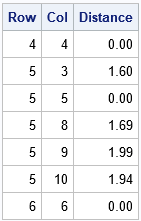
The following statements use the LOC function to locate the elements of D that satisfy the cutoff criterion. (You should always check that the vector returned by the LOC function is nonempty before you use it.) The NDX2SUBS function converts indices into (row, col) subscripts. The subscripts are for the smaller block matrix, so you have to map them to the row numbers in the full distance matrix:

/* Extract elements that satisfy the criterion */
idx = loc( D < cutoff );            /* find elements that satisfy cutoff criterion */
*if ncol(idx) > 0 then do;          /* should check that idx is not empty */
   Distance = D[idx];               /* extract close distances */
   s = ndx2sub(dimension(D), idx);  /* s contains matrix subscripts */
   Row = rows[s[,1]];               /* convert rows to row numbers for full matrix */
   Col = s[,2];          
   print Row Col Distance[F=5.2];

Because the distance matrix is symmetric (and we can exclude the diagonal elements, which are 0), let's agree to report only the upper-triangular portion of the (full) distance matrix. Again, you can use the LOC function to find the (Row, Col) pairs for which Row is strictly less than Col. Those are the pairs of observations that we want to store:

   /* filter: output only upper triangular when full matrix is symmetric */
   k = loc( Row < Col );               /* store only upper triangular in full */
   *if ncol(k)>0 then do;              /* should check that k is not empty */
      Row = Row[k];
      Col = Col[k];
      Distance = Distance[k];
      print Row Col Distance[F=5.2];

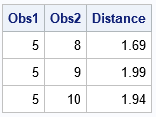
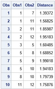
Success! The printed observations are the elements of the upper-triangular distance matrix that satisfy the cutoff criterion. If you repeat these computations for other blocks (observations 1-3, 4-6, 7-9, 10-12, and 13) then you can compute all pairs of observations that are less than 2 units from each other. For the record, here are the 10 pairs of observations that are within 0.5 units of each other. Although the point of this article is to avoid computing the full 13 x 13 distance matrix, for this small example you can check the following table by visual inspection of the full distance matrix, F = distance(X, X).

Block computations to compute distances in large data

The previous section describes the main ideas about using block matrix computations to perform distance computations for large data when the whole N x N distance matrix will not fit into memory. The same ideas apply to cosine similarity and or other pairwise computations. For various reasons, I recommend that the size of the block matrices be less than 2 GB.

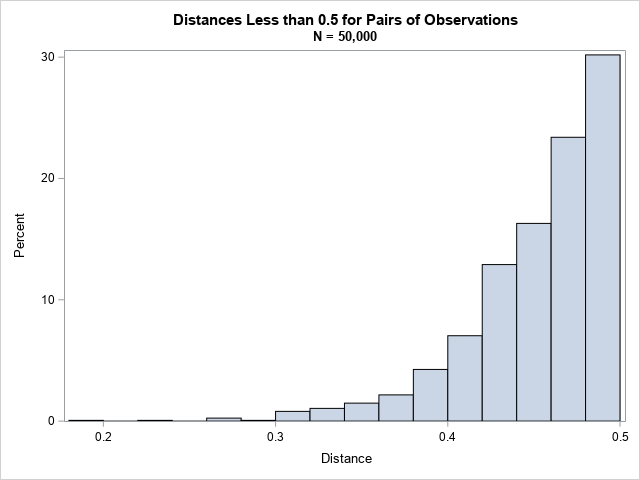
The following DATA step generates 50,000 observations, which means there are 2.5 billion pairs of observations. The program computes all pairwise distances and finds all pairs that are within 0.5 units. The full distance matrix is about 18.6 GB, but the program never computes the full matrix. Instead, the program uses a block size of 5,000 rows and computes a total of 10 distance matrices, each of which requires 1.86 GB of RAM. (See "How much RAM do I need to store that matrix?) For each of these block matrices, the program finds and writes the pairs of observations that are closer than 0.5 units. The program requires about a minute to run on my desktop PC. If you have a slow PC, you might want to use N=20000 to run the example.

/* Create 10 variables and a large number (N) of obs. The complete 
   distance matrix requires N^2 elements. */
%let N = 50000;
data Have;
call streaminit(12345);
array x[10];
do i = 1 to &N;
   do j = 1 to dim(x);  x[j] = rand("Uniform", -1, 1);  end;
   output;
end;
keep x:;
run;
 
/* Find pairs of observations that within 'cutoff' of each other.
   Write these to a data set. */
proc iml;
use Have; read all var _NUM_ into X; close;
n = nrow(X);                    /* number of observations */
m = 5000;                       /* block size: best if n*m elements fit into 2 GB RAM */
cutoff = 0.5;                   /* report pairs where distance < cutoff */
 
startRow = 1;
/* set up output data set to store results */
create Results var {'Obs1' 'Obs2' 'Distance'};
do while (startRow <= n);
   /* Block matrix X = [A1, A2, A3, ..., Ak]  */
   endRow = min(startRow + m - 1, n);  /* don't exceed size of matrix */
   rows = startRow:endRow;
   /* Compute D_i = distance(Ai, X)         */
   A = X[rows,];                /* extract block */
   D = distance(A, X);          /* compute all distances for obs in block */
 
   /* Extract elements that satisfy the criterion */
   idx = loc( D < cutoff );     /* find elements that satisfy cutoff criterion */
   if ncol(idx) > 0 then do;
      Distance = D[idx];        /* extract close distances */
      s = ndx2sub(dimension(D), idx);  /* s contains matrix subscripts */
      Row = rows[s[,1]];        /* convert rows to row numbers for full matrix */ 
      Col = s[,2];          
      /* filter: output only upper triangular when full matrix is symmetric */
      k = loc( Row < Col );     /* store only upper triangular in full */
      if ncol(k)>0 then do;
         Obs1 = Row[k]; Obs2 = Col[k]; Distance = Distance[k];
         append;                /* Write results to data set */
      end;
   end;
   startRow = startRow + m;
end;
close;
QUIT;
 
title "Distances Less than 0.5 for Pairs of Observations";
title2 "N = 50,000";
proc sgplot data=Results;
   histogram Distance;
run;

From the 2.5 billion distances between pairs of observations, the program found 1620 pairs that are closer than 0.5 units in a 10-dimensional Euclidean space. The distribution of those distances is shown in the following histogram.

Further improvements

When the full matrix is symmetric, as in this example, you can improve the algorithm. Because only the upper triangular elements are relevant, you can improve the efficiency of the algorithm by skipping computations that are in the lower triangular portion of the distance matrix.

The k_th block matrix, A, represents consecutive rows in the matrix X. Let L be the row number of the first row of X that is contained in A. You do not need to compute the distance between rows of A and all rows of X. Instead, set Y = X[L:N, ] and compute distance(A, Y). With this modification, you need additional bookkeeping to map the column numbers in the block computation to the column numbers in the full matrix. However, for large data sets, you decrease the computational time by almost half. I leave this improvement as an exercise for the motivated reader.

Conclusions

In summary, you can use a matrix langue like SAS/IML to find pairs of observations that are close to (or far from) each other. By using block-matrix computations, you never have to compute the full N x N distance matrix. Instead, you can compute smaller pieces of the matrix and find the pairs of observations that satisfy your search criterion.

Because this problem is quadratic in the number of observations, you can expect the program to take four times as long if you double the size of the input data. So the program in this article will take about four minutes for 100,000 observations and 16 minutes for 200,000 computations. If that seems long, remember that with 200,000 observations, the program must compute 40 billion pairwise distances.