In simulation studies, sometimes you need to simulate outliers. For example, in a simulation study of regression techniques, you might want to generate outliers in the explanatory variables to see how the technique handles high-leverage points. This article shows how to generate outliers in multivariate normal data that are a specified distance from the center of the distribution. In particular, you can use this technique to generate "regular outliers" or "extreme outliers."

When you simulate data, you know the data-generating distribution. In general, an outlier is an observation that has a small probability of being randomly generated. Consequently, outliers are usually generated by using a different distribution (called the contaminating distribution) or by using knowledge of the data-generating distribution to construct improbable data values.

The geometry of multivariate normal data

A canonical example of adding an improbable value is to add an outlier to normal data by creating a data point that is k standard deviations from the mean. (For example, k = 5, 6, or 10.) For multivaraite data, an outlier does not always have extreme values in all coordinates. However, the idea of an outliers as "far from the center" does generalize to higher dimensions. The following technique generates outliers for multivariate normal data:

1. Generate uncorrelated, standardized, normal data.
2. Generate outliers by adding points whose distance to the origin is k units. Because you are using standardized coordinates, one unit equals one standard deviation.
3. Use a linear transformation (called the Cholesky transformation) to produce multivariate normal data with a desired correlation structure.

In short, you use the Cholesky transformation to transform standardized uncorrelated data into scaled correlated data. The remarkable thing is that you can specify the covariance and then directly compute the Cholesky transformation that will result in that covariance. This is a special property of the multivariate normal distribution. For a discussion about how to perform similar computations for other multivariate distributions, see Chapter 9 in Simulating Data with SAS (Wicklin 2013).

Let's illustrate this method by using a two-dimensional example. The following SAS/IML program generates 200 standardized uncorrelated data points. In the standardized coordinate system, the Euclidean distance and the Mahalanobis distance are the same. It is therefore easy to generate an outlier: you can generate any point whose distance to the origin is larger than some cutoff value. The following program generates outliers that are 5 units from the origin:

ods graphics / width=400px height=400px attrpriority=none;
proc iml;
/* generate standardized uncorrelated data */
call randseed(123);
N = 200;
x = randfun(N//2, "Normal"); /* 2-dimensional data. X ~ MVN(0, I(2)) */
 
/* covariance matrix is product of diagonal (scaling) and correlation matrices.
   See https://blogs.sas.com/content/iml/2010/12/10/converting-between-correlation-and-covariance-matrices.html
 */
R = {1   0.9,             /* correlation matrix */
     0.9 1  };
D = {4 9};                /* standard deviations */
Sigma = corr2cov(R, D);   /* Covariance matrix Sigma = D*R*D */
print Sigma;
 
/* U is the Cholesky transformation that scales and correlates the data */
U = root(Sigma);
 
/* add a few unusual points (outliers) */
pi = constant('pi');
t = T(0:11) * pi / 6;            /* evenly spaced points in [0, 2p) */
outliers = 5#cos(t) || 5#sin(t); /* evenly spaced on circle r=5 */
v = x // outliers;               /* concatenate MVN data and outliers */
w = v*U;                         /* transform from stdized to data coords */
 
labl = j(N,1," ") // T('0':'11');
Type = j(N,1,"Normal") // j(12,1,"Outliers");
title "Markers on Circle r=5";
title2 "Evenly spaced angles t[i] = i*pi/6";
call scatter(w[,1], w[,2]) grid={x y} datalabel=labl group=Type;

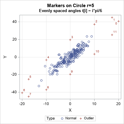
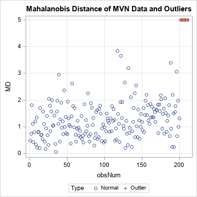
The program simulates standardized uncorrelated data (X ~ MVN(0, I(2))) and then appends 12 points on the circle of radius 5. The Cholesky transformation correlates the data. The correlated data are shown in the scatter plot. The circle of outliers has been transformed into an ellipse of outliers. The original outliers are 5 Euclidean units from the origin; the transformed outliers are 5 units of Mahalanobis distance from the origin, as shown by the following computation:

center = {0 0};
MD = mahalanobis(w, center, Sigma);     /* compute MD based on MVN(0, Sigma) */
obsNum = 1:nrow(w);
title "Mahalanobis Distance of MVN Data and Outliers";
call scatter(obsNum, MD) grid={x y} group=Type;

Adding outliers at different Mahalanobis distances

The same technique enables you to add outliers at any distance to the origin. For example, the following modification of the program adds outliers that are 5, 6, and 10 units from the origin. The t parameter determines the angular position of the outlier on the circle:

MD = {5, 6, 10};               /* MD for outlier */
t = {0, 3, 10} * pi / 6;       /* angular positions */
outliers = MD#cos(t) ||  MD#sin(t);
v = x // outliers;             /* concatenate MVN data and outliers */
w = v*U;                       /* transform from stdized to data coords */
 
labl = j(N,1," ") // {'p1','p2','p3'};
Type = j(N,1,"Normal") // j(nrow(t),1,"Outlier");
call scatter(w[,1], w[,2]) grid={x y} datalabel=labl group=Type;

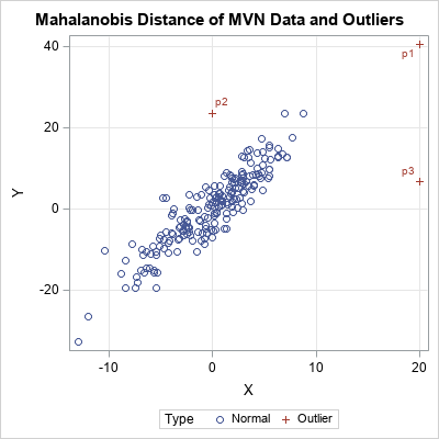
If you use the Euclidean distance, the second and third outliers (p2 and p3) are closer to the center of the data than p1. However, if you draw the probability ellipses for these data, you will see that p1 is more probable than p2 and p3. This is why the Mahalanobis distance is used for measuring how extreme an outlier is. The Mahalanobis distances of p1, p2, and p3 are 5, 6, and 10, respectively.

Adding outliers in higher dimensions

In two dimensions, you can use the formula (x(t), y(t)) = r*(cos(t), sin(t)) to specify an observation that is r units from the origin. If t is chosen randomly, you can obtain a random point on the circle of radius r. In higher dimensions, it is not easy to parameterize a sphere, which is the surface of an d-dimensional ball. Nevertheless, you can still generate random points on a d-dimensional sphere of radius r by doing the following:

1. Generate a point from the d-dimensional multivariate normal distribution: Y = MVN(0, I(d)).
2. Project the point onto the surface of the d-dimensional sphere of radius r: Z = r*Y / ||Y||.
3. Use the Cholesky transformation to correlate the variables.

In the SAS/IML language, it would look like this:

/* General technique to generate random outliers at distance r */
d = 2;                              /* use any value of d */
MD = {5, 6, 10};                    /* MD for outlier */
Y = randfun(nrow(MD)//d, "Normal"); /* d-dimensional Y ~ MVN(0, I(d)) */
outliers = MD # Y / sqrt(Y[,##]);   /* surface of spheres of radii MD */
/* then append to data, use Cholesky transform, etc. */

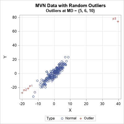
For these particular random outliers, the largest outliers (MD=10) is in the upper right corner. The others are in the lower left corner. If you change the random number seed in the program, the outliers will appear in different locations.

In summary, by understanding the geometry of multivariate normal data and the Cholesky transformation, you can manufacture outliers in specific locations or in random locations. In either case, you can control whether you are adding a "near outlier" or an "extreme outlier" by specifying an arbitrary Mahalanobis distance.

You can download the SAS program that generates the graphs in this article.