How can you generate data that contains outliers in a simulation study? The contaminated normal distribution is a simple but useful distribution you can use to simulate outliers. The distribution is easy to explain and understand, and it is also easy to implement in SAS.

What is a contaminated normal distribution?

The contaminated normal distibution was originally studied by John Tukey in the 190s and '50s. As I say in my book Simulating Data with SAS (2013, p. 119), "the contaminated normal distribution is a specific instance of a two-component mixture distribution in which both components are normally distributed with a common mean.... This results in a distribution with heavier tails than normality. This is also a convenient way to generate data with outliers."

Specifically, a contaminated normal distribution is a mixture of two normal distributions with mixing probabilities (1 - α) and α, where typically 0 < α ≤ 0.1. You can write the density of a contaminated normal distribution in terms of the component densities. Let φ(x; μ, σ) denote the distribution of the normal distribution with mean μ and standard deviation σ. Then the contaminated normal density is
f(x) = (1 - α)φ(x; μ, σ) + α φ(x; μ, λσ)
where λ > 1 is a parameter that determines the standard deviation of the wider component.

The idea is that the "main" distribution (φ(x; μ, σ)) is slightly "contaminated" by a wider distribution. Tukey (1960) uses λ=3 as a scale multiplier. This article uses α = 0.1, which represents 10% "contamination." Tukey reports that when λ=3 and α=0.1, "the two constituents contribute equal amounts to the variance of the contaminated distribution." In the following sections, μ=0 and σ=1, so that the uncontaminated component is the standard normal distribution.

The density of the contaminated normal distribution

The following SAS DATA step constructs the density of a contaminated normal distribution as the linear combination of a N(0,1) and a N(0,3) density. The call to the SGPLOT procedure plots the density and the component densities:

%let alpha = 0.1;
%let lambda = 3;
data CNPDF;
label Y1="N(0,1)" Y2="N(0,3)";
do x = -3*&lambda to 3*&lambda by 0.1;
   Y1 = pdf("Normal", x, 0, 1);             /* std normal component */
   Y2 = pdf("Normal", x, 0, 1*&lambda);     /* contamination */
   CN = (1-&alpha)*Y1 + &alpha*Y2;          /* contaminated normal */
   output;
end;
run;
 
title "Contaminated Normal Distribution";
title2 "alpha = α lambda = &lambda";
proc sgplot data=CNPDF;
   label CN = "0.9 N(0,1) + 0.1 N(0,3)";
   series x=x y=Y1;
   series x=x y=Y2;
   series x=x y=CN / lineattrs=(thickness=3);
   xaxis grid values=(-9 to 9);
   yaxis grid;
run;

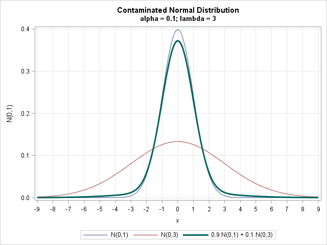
As shown in the graph, the contaminated normal distribution (shown with a thick line) has heavier tails than the "uncontaminated" normal component.

Random samples from the contaminated normal distribution

The book Simulating Data with SAS (2013, p. 120) provides an algorithm for simulating data from a contaminated normal distribution. The algorithm is a special case of simulating from a mixture distribution. You iteratively choose a component with probability α and then generate a value from whichever component is chosen, as follows:

%let alpha= 0.1;               /* level of contamination */
%let lambda = 3;               /* magnitude of contamination */
%let N = 100;                  /* size of sample */
data CNRand(keep=x contaminate);
call streaminit(12345);
do i = 1 to &N;
   contaminate = rand("Bernoulli", &alpha);
   if contaminate then
      x = rand("Normal", 0, &lambda);
   else
      x = rand("Normal", 0, 1);
   output;
end;
run;
 
proc sgplot data=CNRand;
   histogram x;
   density x / type=normal(mu=0 sigma=1) name="normal";
   density x / type=kernel name="kernel";
   fringe x / group=contaminate  lineattrs=(thickness=2);
   keylegend "kernel" "normal" / location=inside position=topright across=1;
   yaxis offsetmin=0.035;
run;

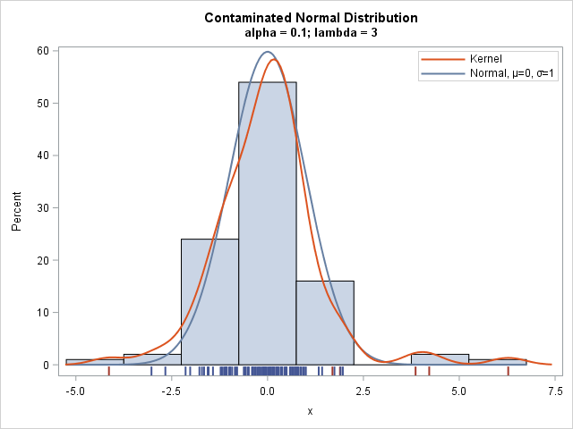
The histogram shows the distribution of the simulated sample. A kernel density estimate is overlaid, as is the density for the uncontaminated N(0,1) component. A fringe plot (also called a "rug plot") is shown underneath the histogram so that you can see the actual values in the sample.

The data that are generated by the uncontaminated component are shown in one color; the data from the contaminated component are shown in a different color. Whereas the standard normal density rarely produces data values for which |x| > 3, the sample contains four values that exceed 3 in magnitude. As you can see, all four "extreme" values are generated from the contaminated component. However, the contaminated component also generates two values that are not so extreme.

CDF and quantiles for the contaminated normal distribution

You can easily compute the cumulative distribution (and therefore probabilities) of the contaminated normal (CN) distribution as a linear combination of the component CDFs. For example, if you want to know the probability that a random observation from the CN distribution exceeds 3 in magnitude, you can compute that probability as follows:

data Prob;
   x = 3;
   leftP  = (1-&alpha)*cdf("Normal", -x, 0, 1) +
                &alpha*cdf("Normal", -x, 0, &lambda);
   totalP = 2*leftP;     /* distribution is symmetric */
run;
proc print noobs;run;

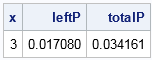
The table shows that the probability is 0.034. Almost all of that probability comes from the contaminated component of the distribution.

The quantile function of the CN distribution does not have a closed-form solution. Given a probability P, the quantile of the CN is the value of x for which P = (1-α)CDF(x; μ, σ) + αCDF(x ; μ, λσ). You can use a root-finding method to find the quantile. For example, you can use the FROOT function in SAS/IML, as follows:

proc iml;
start CNQuantile(x) global (alpha, lambda, Prob);
   return Prob - ( (1-alpha)*CDF("Normal", x, 0, 1) + 
                      alpha *CDF("Normal", x, 0, lambda) );
finish;
 
Prob = 0.01708;
alpha = 0.1;
lambda = 3;
x = froot("CNQuantile", {-9 0});  /* find quantile for Prob */
print x;

The computation find that the quantile for 0.01708 is about -3.

Not all researchers agree that a contaminated normal distribution is an appropriate model for non-Gaussian data. Gleason (1993, JASA) provides an overview of the history of the CN distribution, discusses how the parameters contribute to the elongation of the tail, and compares the CN with other long-tailed distributions.

References

• Gleason, J. R. (1993) "Understanding Elongation: The Scale Contaminated Normal Family," JASA 88(421)
• Tukey, J. W. (1960), “A Survey of Sampling from Contaminated Distributions,” in I. Olkin, ed., Contributions to Probability and Statistics
• Wicklin, R. (2013), Simulating Data with SAS