When solving optimization problems, it is harder to specify a constrained optimization than an unconstrained one. A constrained optimization requires that you specify multiple constraints. One little typo or a missing minus sign can result in an infeasible problem or a solution that is unrelated to the true problem. This article shows two ways to check that you've correctly specified the constraints for a two-parameter optimization. The first is a program that translates the linear constraint matrix in SAS/IML software into a system of linear equations in slope-intercept form. The second is a visualization of the constraint region.

For simplicity, this article only discusses two-dimensional constraint regions. For these regions, the SAS/IML constraint matrix is a k x 4 matrix. We also assume that the constraints are linear inequalities that define a 2-D feasible region.

The SAS/IML matrix for boundary and linear constraints

In SAS/IML software you must translate your boundary and linear constraints into a matrix that encodes the constraints. (The OPTMODEL procedure in SAS/OR software uses a more natural syntax to specify constraints.) The first and second rows of the constraint matrix specify the lower and upper bounds, respectively, for the variables. The remaining rows specify the linear constraints. In general, when you have p variables, the first p columns contain a matrix of coefficients; the (p+1)st column encodes whether the constraint is an equality or inequality; the (p+2)th column specifies the right-hand side of the linear constraints. In this article, p = 2.

The following matrix is similar to the one used in a previous article about how to find an initial guess in a feasible region. The matrix encodes three inequality constraints for a two-parameter optimization. The first two rows of the first column specify bounds for the first variable: 0 ≤ x ≤ 10. The first two rows of the second column specify bounds for the second variable: 0 ≤ y ≤ 8. The third through fifth rows specify linear inequality constraints, as indicated in the comments. The third column encodes the direction of the inequality constraints. A value of -1 means "less than"; a value of +1 means "greater than." You can also use the value 0 to indicate an equality constraint.

proc iml;
con = {  0   0   .   .,        /* lower bounds */
        10   8   .   .,        /* upper bounds */
         3  -2  -1  10,        /* 3*x1 + -2*x2 LE 10 */
         5  10  -1  56,        /* 5*x1 + 10*x2 LE 56 */
         4   2   1   7 };      /* 4*x1 +  2*x2 GE  7 */

Verify the constraint matrix

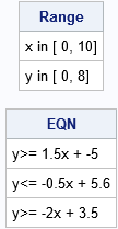
A pitfall of encoding the constraints is that you might wonder whether you made a mistake when you typed the constraint matrix. Also, each linear constraint (row) in the matrix represents a linear equation in "standard form" such as 3*x - 2*y ≤ 10, whereas you might be more comfortable visualizing constraints in the equivalent "slope-intercept form" such as "y ≥ (3/2)x - 5.

It is easy to transform the equations from standard form to slope-intercept form. If c2 > 0, then the standard equation c1*x + c2*y ≥ c0 is transformed to y ≥ (-c1/c2)*x + (c0/c2). If c2 < 0, you need to remember to reverse the sign of the inequality: y ≤ (-c1/c2)*x + (c0/c2). Because the (p+1)th column has values ±1, you can use the SIGN function to perform all transformations without writing a loop. The following function "decodes" the constraint matrix and prints it is "human readable" form:

start BLCToHuman(con);
   nVar = ncol(con) - 2;
   Range = {"x", "y"} + " in [" + char(con[1,1:nVar]`) + "," + char(con[2,1:nVar]`) + "]";
   cIdx = 3:nrow(con);              /* rows for the constraints */
   c1 = -con[cIdx,1] / con[cIdx,2];
   c0 =  con[cIdx,4] / con[cIdx,2];
   sign = sign(con[cIdx,3] # con[cIdx,2]);
   s = {"<=" "=" ">="};
   idx = sign + 2;                 /* convert from {-1 0 1} to {1 2 3} */
   EQN = "y" + s[idx] + char(c1) + "x + " + char(c0);
   print Range, EQN;
finish;
 
run BLCToHuman(con);

Visualize the feasible region

In a previous article, I showed a technique for visualizing a feasible region. The technique is crude but effective. You simply evaluate the constraints at each point of a dense, regular, grid. If a point satisfies the constraints, you plot it in one color; otherwise, you plot it in a different color.

For linear constraints, you can perform this operation by using matrix multiplication. If A is the matrix of linear coefficients and all inequalities are "greater than" constraints, then you simply check that A*X ≥ b, where b is the right-hand side (the (p+2)th column). If any of the inequalities are "less than" constraints, you can multiply that row of the constraint matrix by -1 to convert it into an equivalent "greater than" constraint. This algorithm is implemented in the following SAS/IML function:

start PlotFeasible(con);
   L = con[1, 1:2];                   /* lower bound constraints */
   U = con[2, 1:2];                   /* upper bound constraints */
   cIdx = 3:nrow(con);                /* rows for linear inequality constraints */
   C = con[cIdx,] # con[cIdx,3];      /* convert all inequalities to GT */ 
   M = C[, 1:2];                      /* coefficients for linear constraints */
   RHS = C[, 4];                      /* right hand side */
   x = expandgrid( do(L[1], U[1], (U[1]-L[1])/50),    /* define (x,y) grid from bounds */
                   do(L[2], U[2], (U[2]-L[2])/50) );
   q = (M*x`>= RHS);                  /* 0/1 indicator matrix */
   Feasible = (q[+,] = ncol(cIdx));   /* are all constraints satisfied? */
   call scatter(x[,1], x[,2],) group=Feasible grid={x y} option="markerattrs=(symbol=SquareFilled)";
finish;
 
ods graphics / width=430px height=450px;
title "Feasible Region";
title2 "Formed by Bounds and Linear Constraints";
run PlotFeasible(con);

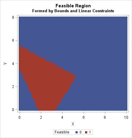
The graph shows that the feasible region as a red pentagonal region. The left and lower edges are determined by the bounds on the parameters. There are three diagonal lines that are determined by the linear inequality constraints. By inspection, you can see that the point (2, 2) is in the feasible region. Similarly, the point (8,6) is in the blue region and is not feasible.

The technique uses the bounds on the parameters (the first two rows) to specify the range of the axes in the plot. If your problem does not have explicit upper/lower bounds on the parameters, you can "invent" bounds such as [0, 100] or [-10, 10] just for plotting the feasible region.

In summary, this article shows two techniques that can help you verify that a constraint matrix is correctly specified. The first translates that constraint matrix into "human readable" form. The second draws a crude approximation of the feasible region by evaluating the constraints at each location on a dense grid. Both techniques are shown for two-parameter problems. However, with a little effort, you could incorporate the second technique when searching for a good initial guess in higher-dimensional problems.