This article shows how to perform an optimization in SAS when the parameters are restricted by nonlinear constraints. In particular, it solves an optimization problem where the parameters are constrained to lie in the annular region between two circles. The end of the article shows the path of partial solutions which converges to the solution and verifies that all partial solutions lie within the constraints of the problem.

The four kinds of constraints in optimization

The term "nonlinear constraints" refers to bounds placed on the parameters. There are four types of constraints in optimization problems. From simplest to most complicated, they are as follows:

• Unconstrained optimization: In this class of problems, the parameters are not subject to any constraints.
• Bound-constrained optimization: One or more parameters are bounded. For example, the scale parameter in a probability distribution is constrained by σ > 0.
• Linearly constrained optimization: Two or more parameters are linearly bounded. In a previous example, I showed images of a polygonal "feasible region" that can result from linear constraints.
• Nonlinearly constrained optimization: Two or more parameters are nonlinearly bounded. This article provides an example.

A nonlinearly constrained optimization

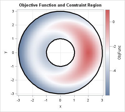
This article solves a two-dimensional nonlinearly constrained optimization problem. The constraint region will be the annular region defined by the two equations
x² + y² ≥ 1
x² + y² ≤ 9

Let f(x,y) be the objective function to be optimized. For this example,
f(x,y) = cos(π r) - Dist( (x,y), (2,0) )
where
r = sqrt(x² + y²) and
Dist( (x,y), (2,0) ) = sqrt( (x-2)² + (y-0)² )
is the distance from (x,y) to the point (2,0).

By inspection, the maximum value of f occurs at (x,y) = (2,0) because the objective function obtains its largest value (1) at that point. The following SAS statements use a scatter plot to visualize the value of the objective function inside the constraint region. The graph is shown to the right.

/* evaluate the objective function on a regular grid */
data FuncViz;
do x = -3 to 3 by 0.05;
   do y = -3 to 3 by 0.05;
      r2 = x**2 + y**2;
      r = sqrt(r2);
      ObjFunc = cos(constant('pi')*r) - sqrt( (x-2)**2+(y-0)**2 );
      if 1 <= r2 <= 9 then output;  /* output points in feasible region */
   end;
end;
run;
 
/* draw the boundary of the constraint region */
%macro DrawCircle(R);
   R = &R;
   do t = 0 to 2*constant('pi') by 0.05; 
      xx= R*cos(t); yy= R*sin(t); output;
   end;
%mend;
data ConstrBoundary;
   %DrawCircle(1)
   %DrawCircle(3)
run;
 
ods graphics / width=400px height=360px antialias=on antialiasmax=12000 labelmax=12000;
title "Objective Function and Constraint Region";
data Viz; set FuncViz ConstrBoundary;  run;
 
proc sgplot data=Viz noautolegend;
   xaxis grid; yaxis grid;
   scatter x=x y=y / markerattrs=(symbol=SquareFilled size=4)
                     colorresponse=ObjFunc colormodel=ThreeColorRamp; 
   polygon ID=R x=xx y=yy / lineattrs=(thickness=3);
   gradlegend;
run;

Solving a constrained optimization problem in SAS/IML

SAS/IML and SAS/OR each provide general-purpose tools for optimization in SAS. This section solves the problem by using SAS/IML. A solution that uses PROC OPTMODEL is more compact and is shown at the end of this article.

SAS/IML supports 10 different optimization algorithms. All support unconstrained, bound-constrained, and linearly constrained optimization. However, only two support nonlinear constraints: the quasi-Newton method (implemented by using the NLPQN subroutine) and the Nelder-Mead simplex method (implemented by using the NLPNMS subroutine).

To specify k nonlinear constraints in SAS/IML, you need to do two things:

• Use the options vector to the NLP subroutines to specify the number of nonlinear constraints. Set optn[10] = k to tell SAS/IML that there are a total of k constraints. If any of the constraints are equality constraints, specify that number in the optn[11] field. That is, if there are k_eq equality constraints, then optn[11] = k_eq.
• Write a SAS/IML module that accepts a parameter value as input and produces a column vector that contains k rows. Each row representing the evaluation of one of the constraints on the input parameters. For consistency, all nonlinear inequality constraints should be written in the form g(c) ≥ 0. The first k_eq rows contains the equality constraints and the remaining k – k_eq elements contain the inequality constraints. You specify the module that evaluates the nonlinear constraints by using the NLC= option on the NLPQN or NLPNMS subroutine.

For the current example, k = 2 and k_eq = 0. Therefore the module that specifies the nonlinear constraints should return two rows. The first row evaluates whether a parameter value is outside the unit circle. The second row evaluates whether a parameter value is inside the circle with radius 3. Both constraints need to be written as "greater than" inequalities. This leads to the following SAS/IML program which solves the nonlinear optimization problem:

proc iml;
start ObjFunc(z);
   r = sqrt(z[,##]);        /* z = (x,y) ==> z[,##] = x##2 + y##2 */
   f = cos( constant('pi')*r ) - sqrt( (z[,1]-2)##2 + (z[,2]-0)##2 ); 
   return f;
finish;
 
start NLConstr(z);
   con = {0, 0};            /* column vector for two constraints */
   con[1] = z[,##] - 1;     /* (x##2 + y##2) >= 1    ==> (x##2 + y##2) - 1 >= 0 */
   con[2] = 9 - z[,##];     /* (x##2 + y##3) <= 3##2 ==> 9 - (x##2 + y##2) >= 0 */
   return con;
finish;
 
optn= j(1,11,.);     /* allocate options vector (missing ==> 'use default') */
optn[1] = 1;         /* maximize objective function */
optn[2] = 4;         /* include iteration history in printed output */
optn[10]= 2;         /* there are two nonlinear constraints */
optn[11]= 0;         /* there are no equality constraints */
 
ods output grad = IterPath;   /* save iteration history in 'IterPath' data set */
z0 = {-2 0};                  /* initial guess */
call NLPNMS(rc,xOpt,"ObjFunc",z0,optn) nlc="NLConstr";   /* solve optimization */
ods output close;

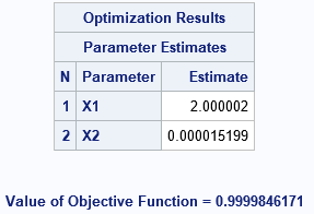
The call to the NLPNMS subroutine generates a lot of output (because optn[2]=4). The final parameter estimates are shown. The routine estimates the optimal parameters as (x,y) = (2.000002, 0.000015), which is very close to the exact optimal value (x,y)=(2,0). The objective function at the estimated parameters is within 1.5E-5 of the true maximum.

Visualizing the iteration path towards an optimum

I intentionally chose the initial guess for this problem to be (x0,y0)=(-2,0), which is diametrically opposite the true value in the annular region. I wanted to see how the optimization algorithm traverses the annular region. I knew that every partial solution would be within the feasible region, but I suspected that it might be possible for the iterates to "jump across" the hole in the middle of the annulus. The following SAS statements visualize the iteration history of the Nelder-Mead method as it iterates towards an optimal solution:

data IterPath2;
   set IterPath;
   Iteration = '  ';
   if _N_ IN (1,5,6,7,9) then Iteration = put(_N_,2.); /* label certain step numbers */
   format Iteration 2.;
run;
 
data Path;  set Viz IterPath2;  run;
 
title "Objective Function and Solution Path";
title2 "Nelder-Mead Simplex Method";
proc sgplot data=Path noautolegend;
   xaxis grid; yaxis grid;
   scatter x=x y=y / markerattrs=(symbol=SquareFilled size=4)
                     colorresponse=ObjFunc colormodel=ThreeColorRamp; 
   polygon ID=R x=xx y=yy / lineattrs=(thickness=3);
   series x=x1 y=x2 / markers datalabel=Iteration datalabelattrs=(size=8) markerattrs=(size=5);
   gradlegend;
run;

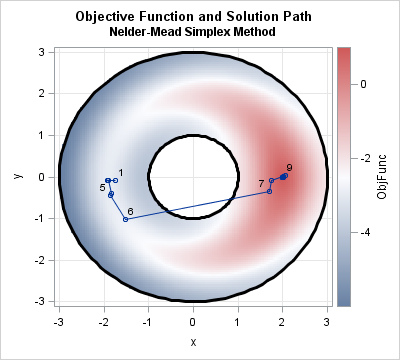
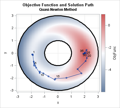
For this initial guess and this optimization algorithm, the iteration path "jumps across" the hole in the annulus on the seventh iteration. For other initial guesses or methods, the iteration might follow a different path. For example, if you change the initial guess and use the quasi-Newton method, the optimization requires many more iterations and follows the "ridge" near the circle of radius 2, as shown below:
z0 = {-2 -0.1}; /* initial guess */
call NLPQN(rc,xOpt,"ObjFunc",z0,optn) nlc="NLConstr"; /* solve optimization */

Nonlinear constraints with PROC OPTMODEL

If you have access to SAS/OR software, PROC OPTMODEL provides a syntax that is compact and readable. For this problem, you can use a single CONSTRAINT statement to specify both the inner and outer bounds of the annular constraints. The following call to PROC OPTMODEL uses an interior-point method to compute a solution that numerically equivalent to (x,y) = (2, 0):

proc optmodel;
   var x, y;
   max f = cos(constant('pi')*sqrt(x^2+y^2)) - sqrt((x-2)^2+(y-0)^2);
   constraint 1 <= x^2 + y^2 <= 9;       /* define constraint region */
   x = -2; y = -0.1;                     /* initial guess */
   solve with NLP / maxiter=25;
   print x y;
quit;

Summary

In summary, you can use SAS software to solve nonlinear optimization problems that are unconstrained, bound-constrained, linearly constrained, or nonlinearly constrained. This article shows how to solve a nonlinearly constrained problem by using SAS/IML or SAS/OR software. In SAS/IML, you have to specify the number of nonlinear constraints and write a function that can evaluate a parameter value and return a vector of positive numbers if the parameter is in the constrained region.