An important application of nonlinear optimization is finding parameters of a model that fit data. For some models, the parameters are constrained by the data. A canonical example is the maximum likelihood estimation of a so-called "threshold parameter" for the three-parameter lognormal distribution. For this distribution, the objective function is the log-likelihood function, which includes a term that looks like log(x_i - θ), where x_i is the i_th data value and θ is the threshold parameter. Notice that you cannot evaluate the objective function for large values of θ. Similar situations occur for other distributions (such as the Weibull) that contain threshold parameters. The domain of the objective function is restricted by the data.

In SAS, you can fit these three-parameter distributions by using PROC UNIVARIATE. However, it is instructive to fit the lognormal distribution "manually" because it illustrates the general problem, which is how to handle optimization for which parameters depend on the data. This article provides two tips. First, you can use boundary constraints to ensure that the optimal solution enforces the condition θ < min(x). Second, you can define the objective function so that it does not attempt to evaluate expressions like log(x_i - θ) if the argument to the LOG function is not positive.

Fit the three-parameter lognormal distribution in SAS

Before discussing the details of optimization, let's look at some data and the MLE parameter estimates for the three-parameter lognormal distribution. The following example is from the PROC UNIVARIATE documentation. The data are measurements of 50 diameters of steel rods that were produced in a factory. The company wants to model the distribution of rod diameters.

data Measures;
   input Diameter @@;
   label Diameter = 'Diameter (mm)';
   datalines;
5.501  5.251  5.404  5.366  5.445  5.576  5.607  5.200  5.977  5.177
5.332  5.399  5.661  5.512  5.252  5.404  5.739  5.525  5.160  5.410
5.823  5.376  5.202  5.470  5.410  5.394  5.146  5.244  5.309  5.480
5.388  5.399  5.360  5.368  5.394  5.248  5.409  5.304  6.239  5.781
5.247  5.907  5.208  5.143  5.304  5.603  5.164  5.209  5.475  5.223
;
 
title 'Lognormal Fit for Diameters';
proc univariate data=Measures noprint;
   histogram Diameter / lognormal(scale=est shape=est threshold=est) odstitle=title;
   ods select ParameterEstimates Histogram;
run;

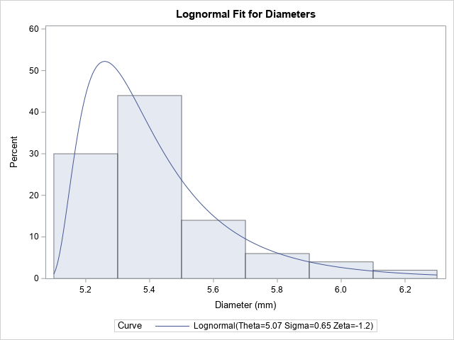
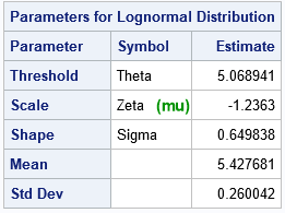
The UNIVARIATE procedure overlays the MLE fit on a histogram of the data. The ParameterEstimates table shows the estimates. The threshold parameter (θ) is the troublesome parameter when you fit models like this. The other two parameters ("Zeta," which I will call μ in the subsequent sections, and σ) are easier to fit.

An important thing to note is that the estimate for the threshold parameter is 5.069. If you look at the data (or use PROC MEANS), you will see that the minimum data value is 5.143. To be feasible, the value of the threshold parameter must always be less than 5.143 during the optimization process. The log-likelihood function is undefined if θ ≥ min(x).

Tip 1: Constrain the domain of the objective function

Although PROC UNIVARIATE automatically fits the three-parameter lognormal distribution, it is instructive to explicitly write the log-likelihood function and solve the optimization problem "manually." Given N observations {x₁, x₂, ..., x_N}, you can use maximum likelihood estimation (MLE) to fit a three-parameter lognormal distribution to the data. I've previously written about how to use the optimization functions in SAS/IML software to carry out maximum likelihood estimation. The following SAS/IML statements define the log-likelihood function:

proc iml;
start LN_LL1(parm) global (x);
   mu = parm[1]; sigma = parm[2]; theta = parm[3];
   n = nrow(x);
   LL1 = -n*log(sigma) - n*log(sqrt(2*constant('pi')));
   LL2 = -sum( log(x-theta) );                         /* not defined if theta >= min(x) */
   LL3 = -sum( (log(x-theta)-mu)##2 ) / (2*sigma##2);
   return LL1 + LL2 + LL3;
finish;

Recall that for MLE problems, the data are constant values that are known before the optimization begins. The previous function uses the GLOBAL statement to access the data vector, x. The log-likelihood function contains three terms, two of which (LL2 and LL3) are undefined for θ ≥ min(x). Most optimization software enables you to specify constraints on the parameters. In the SAS/IML matrix language, you can define a two-row matrix where the first row indicates lower bounds on the parameters and the second row indicates upper bound. For this problem, the upper bound for the θ parameter is set to min(x) – ε, where ε is a small number so that the quantity (x_i - θ) is always bounded away from 0:

use Measures; read all var "Diameter" into x; close;  /* read data */
/* Parameters of the lognormal(mu, sigma, theta):
      mu   sigma>0  theta<min(x)  */   
con = {.    1e-6      .,           /* lower bbounds: sigma > 0 */
       .    .         .};          /* upper bounds */
con[2,3] = min(x) - 1e-6;          /* replace upper bound for theta */
 
/* optimize the log-likelihood function */
x0 = {0 0.5 4};           /* initial guess is not feasible */
opt = {1,                 /* find maximum of function   */
       0};                /* do not display information about optimization */
call nlpnra(rc, result, "LN_LL1", x0, opt) BLC=con;   /* Newton's method with boundary constraints */
print result[c={'mu' 'sigma' 'theta'} L="Optimum"];

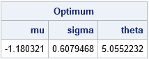
The results are very close to the estimates that were produced by PROC UNIVARIATE. Because of the boundary constraints, the optimization process never evaluates the objective function outside of the feasible domain, as determined by the boundary constraints in the CON matrix.

Tip 2: Trap domain errors in the objective function

Ideally, the log-likelihood function should be robust, meaning that it should be able to handle inputs that are outside of the domain of the function. This enables you to use the objective function in many ways, including visualizing the feasible region and solving problems that have nonlinear constraints. When you have nonlinear constraints, some algorithms might evaluate the function in the infeasible region, so it is important that the objective function does not experience a domain error.

The best way to make the log-likelihood function robust is to trap domain errors. But what value should the software return if an input value is outside the domain of the function?

• If your optimization routine can handle missing values, return a missing value. This is the best mathematical choice because the function cannot be evaluated.
• If your optimization routine does not handle missing values, return a very large value. If you are maximizing the function, return a large negative value such as -1E20. If you are minimizing the function, return a large positive value, such as 1E20. Essentially, this adds a penalty term to the objective function. The penalty is zero when the input is inside the domain and has a large magnitude when the input is outside the domain.

The SAS/IML optimization routines support missing values, so the following module redefines the objective function to return a missing value when θ ≥ min(x):

/* Better: Trap out-of-domain errors to ensure that the objective function NEVER fails */
start LN_LL(parm) global (x);
   mu = parm[1]; sigma = parm[2]; theta = parm[3];
   n = nrow(x);
 
   if theta > min(x) then return .;     /* Trap out-of-domain errors */
 
   LL1 = -n*log(sigma) - n*log(sqrt(2*constant('pi')));
   LL2 = -sum( log(x-theta) );
   LL3 = -sum( (log(x-theta)-mu)##2 ) / (2*sigma##2);
   return LL1 + LL2 + LL3;
finish;

This modified function can be used for many purposes, including optimization with nonlinear constraints, visualization, and so forth.

In summary, this article provides two tips for optimizing a function that has a restricted domain. Often this situation occurs when one of the parameters depends on data, such as the threshold parameter in the lognormal and Weibull distributions. Because the data are constant values that are known before the optimization begins, you can write constraints that depend on the data. You can also access the data during the optimization process to ensure that the objective function does not ever evaluate input values that are outside its domain. If your optimization routine supports missing values, the objective function can return a missing value for invalid input values. Otherwise, the function can return a very large (positive or negative) value for out-of-domain inputs.