A SAS programmer recently asked me how to compute a kernel regression in SAS. He had read my blog posts "What is loess regression" and "Loess regression in SAS/IML" and was trying to implement a kernel regression in SAS/IML as part of a larger analysis. This article explains how to create a basic kernel regression analysis in SAS. You can download the complete SAS program that contains all the kernel regression computations in this article.

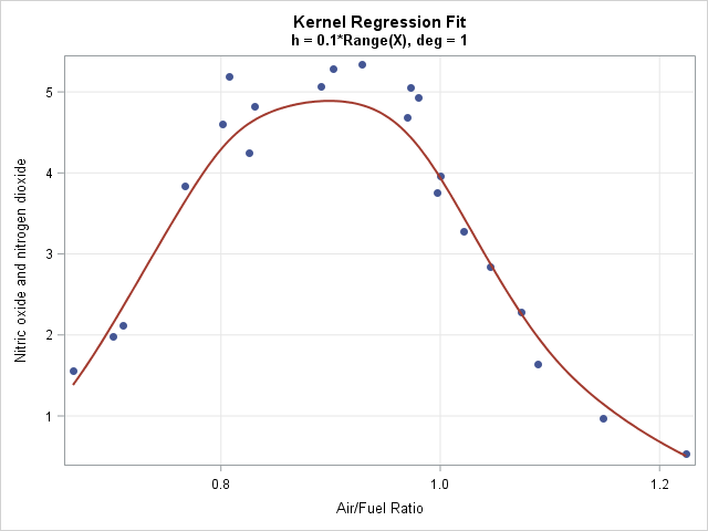
A kernel regression smoother is useful when smoothing data that do not appear to have a simple parametric relationship. The following data set contains an explanatory variable, E, which is the ratio of air to fuel in an engine. The dependent variable is a measurement of certain exhaust gasses (nitrogen oxides), which are contributors to the problem of air pollution. The scatter plot to the right displays the nonlinear relationship between these variables. The curve is a kernel regression smoother, which is developed later in this article.

data gas;
label NOx = "Nitric oxide and nitrogen dioxide";
label E = "Air/Fuel Ratio";
input NOx E @@;
datalines;
4.818  0.831   2.849  1.045   3.275  1.021   4.691  0.97    4.255  0.825
5.064  0.891   2.118  0.71    4.602  0.801   2.286  1.074   0.97   1.148
3.965  1       5.344  0.928   3.834  0.767   1.99   0.701   5.199  0.807
5.283  0.902   3.752  0.997   0.537  1.224   1.64   1.089   5.055  0.973
4.937  0.98    1.561  0.665
;

What is kernel regression?

Kernel regression was a popular method in the 1970s for smoothing a scatter plot. The predicted value, ŷ₀, at a point x₀ is determined by a weighted polynomial least squares regression of data near x₀. The weights are given by a kernel function (such as the normal density) that assigns more weight to points near x₀ and less weight to points far from x₀. The bandwidth of the kernel function specifies how to measure "nearness." Because kernel regression has some intrinsic problems that are addressed by the loess algorithm, many statisticians switched from kernel regression to loess regression in the 1980s as a way to smooth scatter plots.

Because of the intrinsic shortcomings of kernel regression, SAS does not have a built-in procedure to fit a kernel regression, but it is straightforward to implement a basic kernel regression by using matrix computations in the SAS/IML language. The main steps for evaluating a kernel regression at x₀ are as follows:

1. Choose a kernel shape and bandwidth (smoothing) parameter: The shape of the kernel density function is not very important. I will choose a normal density function as the kernel. A small bandwidth overfits the data, which means that the curve might have lots of wiggles. A large bandwidth tends to underfit the data. You can specify a bandwidth (h) in the scale of the explanatory variable (X), or you can specify a value, H, that represents the proportion of the range of X and then use h = H*range(X) in the computation. A very small bandwidth can cause the kernel regression to fail. A very large bandwidth causes the kernel regression to approach an OLS regression.
2. Assign weights to the nearby data: Although the normal density is infinite in support, in practice, observations farther than five bandwidths from x₀ get essentially zero weight. You can use the PDF function to easily compute the weights. In the SAS/IML language, you can pass a vector of data values to the PDF function and thus compute all weights in a single call.
3. Compute a weighted regression: The predicted value, ŷ₀, of the kernel regression at x₀ is the result of a weighted linear regression where the weights are assigned as above. The degree of the polynomial in the linear regression affects the result. The next section shows how to compute a first-degree linear regression; a subsequent section shows a zero-degree polynomial, which computes a weighted average.

Implement kernel regression in SAS

To implement kernel regression, you can reuse the SAS/IML modules for weighted polynomial regression from a previous blog post. You use the PDF function to compute the local weights. The KernelRegression module computes the kernel regression at a vector of points, as follows:

proc iml;
/* First, define the PolyRegEst and PolyRegScore modules 
   https://blogs.sas.com/content/iml/2016/10/05/weighted-regression.html 
   See the DOWNLOAD file.   
*/
 
/* Interpret H as "proportion of range" so that the bandwidth is h=H*range(X)
   The weight of an observation at x when fitting the regression at x0 
   is given by the f(x; x0, h), which is the density function of N(x0, h) at x.
   This is equivalent to (1/h)*pdf("Normal", (X-x0)/h) for the standard N(0,1) distribution. */
start GetKernelWeights(X, x0, H);
   return pdf("Normal", X, x0, H*range(X));   /* bandwidth h = H*range(X) */
finish;
 
/* Kernel regression module. 
   (X,Y) are column vectors that contain the data.
   H is the proportion of the data range. It determines the 
     bandwidth for the kernel regression as h = H*range(X)
   t is a vector of values at which to evaluate the fit. By defaul t=X.
*/
start KernelRegression(X, Y, H, _t=X, deg=1);
   t = colvec(_t);
   pred = j(nrow(t), 1, .);
   do i = 1 to nrow(t);
      /* compute weighted regression model estimates, degree deg */
      W = GetKernelWeights(X, t[i], H);
      b = PolyRegEst(Y, X, W, deg);    
      pred[i] = PolyRegScore(t[i], b);  /* score model at t[i] */
   end;
   return pred;
finish;

The following statements load the data for exhaust gasses and sort them by the X variable (E). A call to the KernelRegression module smooths the data at 201 evenly spaced points in the range of the explanatory variable. The graph at the top of this article shows the smoother overlaid on a scatter plot of the data.

use gas;  read all var {E NOx} into Z;  close;
call sort(Z);   /* for graphing, sort by X */
X = Z[,1];  Y = Z[,2];
 
H = 0.1;        /* choose bandwidth as proportion of range */
deg = 1;        /* degree of regression model */
Npts = 201;     /* number of points to evaluate smoother */
t = T( do(min(X), max(X), (max(X)-min(X))/(Npts-1)) ); /* evenly spaced x values */
pred =  KernelRegression(X, Y, H, t);                  /* (t, Pred) are points on the curve */

Nadaraya–Watson kernel regression

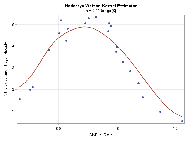
If you use a degree-zero polynomial to compute the smoother, each predicted value is a locally-weighted average of the data. This smoother is called the Nadaraya–Watson (N-W) kernel estimator. Because the N-W smoother is a weighted average, the computation is much simpler than for linear regression. The following two modules show the main computation. The N-W kernel smoother on the same exhaust data is shown to the right.

/* Nadaraya-Watson kernel estimator, which is a locally weighted average */
start NWKerReg(Y, X, x0, H);
   K = colvec( pdf("Normal", X, x0, H*range(X)) );
   return( K`*Y / sum(K) );
finish;
 
/* Nadaraya-Watson kernel smoother module. 
   (X,Y) are column vectors that contain the data.
   H is the proportion of the data range. It determines the 
     bandwidth for the kernel regression as h = H*range(X)
   t is a vector of values at which to evaluate the fit. By default t=X.
*/
start NWKernelSmoother(X, Y, H, _t=X);
   t = colvec(_t);
   pred = j(nrow(t), 1, .);
   do i = 1 to nrow(t);
      pred[i] = NWKerReg(Y, X, t[i], H);
   end;
   return pred;
finish;

Problems with kernel regression

As mentioned earlier, there are some intrinsic problems with kernel regression smoothers:

• Kernel smoothers treat extreme values of a sample distribution differently than points near the middle of the sample. For example, if x₀ is the minimum value of the data, the fit at x₀ is a weighted average of only the observations that are greater than x₀. In contrast, if x₀ is the median value of the data, the fit is a weighted average of points on both sides of x₀. You can see the bias in the graph of the Nadaraya–Watson estimate, which shows predicted values that are higher than the actual values for the smallest and largest values of the X variable. Some researchers have proposed modified kernels to handle this problem for the N-W estimate. Fortunately, the local linear estimator tends to perform well.
• The bandwidth of kernel smoothers cannot be too small or else there are values of x₀ for which prediction is not possible. If d = x[i+1] – x[i]is the gap between two consecutive X data values, then if h is smaller than about d/10, there is no way to predict a value at the midpoint (x[i+1] + x[i]) / 2. The linear system that you need to solve will be singular because the weights at x₀ are zero. The loess method avoids this flaw by using nearest neighbors to form predicted values. A nearest-neighbor algorithm is a variable-width kernel method, as opposed to the fixed-width kernel used here.

Extensions of the simple kernel smoother

You can extend the one-dimensional example to more complex situations:

• Higher Dimensions: You can compute kernel regression for two or more independent variables by using a multivariate normal density as the kernel function. In theory, you could use any correlated structure for the kernel function, but in practice most people use a covariance structure of the form Σ = diag(h²₁, ..., h²_k), where h_i is the bandwidth in the i_th coordinate direction. An even simpler covariance structure is to use the same bandwidth in all directions, which can be evaluated by using the one-dimensional standard normal density evaluated at || x - x₀ || / h. Details are left as an exercise.
• Automatic selection of the bandwidth: The example in this article uses a specified bandwidth, but as I have written before, it is better to use a fit criterion such as GCV or AIC to select a smoothing parameter.

In summary, you can use a weighted polynomial regression to implement a kernel smoother in SAS. The weights are provided by a kernel density function, such as the normal density. Implementing a simple kernel smoother requires only a few statements in the SAS/IML matrix language. However, most modern data analysts prefer a loess smoother over a kernel smoother because the loess algorithm (which is a varying-width kernel algorithm) solves some of the issues that arise when trying to use a fixed-width kernel smoother with a small bandwidth. You can use PROC LOESS in SAS to compute a loess smoother.