What is weighted regression? How does it differ from ordinary (unweighted) regression? This article describes how to compute and score weighted regression models.

Visualize a weighted regression

Technically, an "unweighted" regression should be called an "equally weighted " regression since each ordinary least squares (OLS) regression weights each observation equally. Similarly, an "unweighted mean" is really an equally weighted mean.

Recall that weights are not the same as frequencies. When talking about weights, it is often convenient to assume that the weights sum to unity. This article uses standardized weights, although you can use specify any set of weights when you use a WEIGHT statement in a SAS procedure.

One way to look at a weighted regression is to assume that a weight is related to the variance of an observation. Namely, the i_th weight, w_i, indicates that the variance of the i_th value of the dependent variable is σ² / w_i, where σ² is a common variance. Notice that an observation that has a small weight (near zero) has a relatively large variance. Intuitively, the observed response is not known with much precision; a weighted analysis makes that observation less influential.

For example, the following SAS data set defines (x,y) values and weights (w) for 11 observations. Observations whose X value is close to x=10 have relatively large weights. Observations far from x=10 have small weights. The last observation (x=14) is assigned a weight of zero, which means that it will be completely excluded from the analysis.

data RegData;
input y x w;
datalines;
2.3  7.4  0.058 
3.0  7.6  0.073 
2.9  8.2  0.114 
4.8  9.0  0.144 
1.3 10.4  0.151 
3.6 11.7  0.119 
2.3 11.7  0.119 
4.6 11.8  0.114 
3.0 12.4  0.073 
5.4 12.9  0.035 
6.4 14.0  0 
;

You can use PROC SGPLOT to visualize the observations and weights. In fact, PROC SGPLOT supports a REG statement that adds a regression line to the plot. The REG statement supports adding both weighted and unweighted regression lines:

proc sgplot data=RegData;
scatter x=x y=y / filledoutlinedmarkers markerattrs=(size=12 symbol=CircleFilled)
                colorresponse=w colormodel=TwoColorRamp;     /* color markers by weight */
reg x=x y=y / nomarkers legendlabel="Unweighted Regression"; /* usual OLS regression */
reg x=x y=y / weight=w nomarkers legendlabel="Weighted Regression"; /* weighted regression */
xaxis grid; yaxis grid;
run;

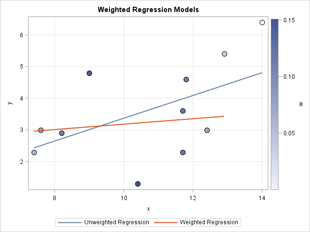
Each marker is colored by its weight. Dark blue markers (observations for which 8 < x < 12) have relatively large weights. Light blue markers have small weights and do not affect the weighted regression model very much.

You can see the effect of the weights by comparing the weighted and unweighted regression lines. The unweighted regression line (in blue) is pulled upward by the observations near x=13 and x=14. These observations have small weights, so the weighted regression line (in red) is not pulled upwards.

Weighted regression by using PROC REG

If you want to compute parameter estimates and other statistics, you can use the REG procedure in SAS/STAT to run the weighted and unweighted regression models. The following statement run PROC REG twice: once without a WEIGHT statement and once with a WEIGHT statement:

proc reg data=RegData plots(only)=FitPlot;
   Unweighted: model y = x;
   ods select NObs ParameterEstimates  FitPlot;
quit;
 
proc reg data=RegData plots(only)=FitPlot;
   Weighted: model y = x;
   weight w;
   ods select NObs ParameterEstimates  FitPlot;
quit;

The output (not shown) indicates that the unweighted regression model is Y = -0.23 + 0.36*X. In contrast, the weighted regression model is Y = 2.3 + 0.085*X. This confirms that the slope of the weighted regression line is smaller than the slope of the unweighted line.

A weighted regression module in SAS/IML

You can read the SAS documentation to find the formulas that are used for a weighted OLS regression model. The formula for the parameter estimates is a weighted version of the normal equations: b = (X`WX)<sup>-1</sup>(X`WY), where Y is the vector of observed responses, X is the design matrix, and W is the diagonal matrix of weights.

In SAS/IML it is more efficient to use elementwise multiplication than to multiply with a diagonal matrix. If you work through the matrix equations, you will discover that weighted regression is easily accomplished by using the normal equations on the matrices that result from multiplying the rows of Y and X by the square root of the weights. This is implemented in the following SAS/IML module:

proc  iml;
/* weighted polynomial regression for one regressor. Y, X, and w are col vectors */
start PolyRegEst(Y, X, w, deg);
   Yw = sqrt(w)#Y;                  /* mult rows of Y by sqrt(w) */
   XDesign = j(nrow(X), deg+1);
   do j = 0 to deg;                 /* design matrix for polynomial regression */
      Xdesign[,j+1] = X##j;
   end;
   Xw = sqrt(w)#Xdesign;            /* mult rows of X by sqrt(w) */
   b = solve(Xw`*Xw, Xw`*Yw);       /* solve normal equation */
   return b;
finish;
 
use RegData; read all var {Y X w}; close;    /* read data and weights */
 
/* loop to perform one-variable polynomial regression for deg=0, 1, and 2 */
do deg = 0 to 2;                    
   b = PolyRegEst(Y, X, w, deg);
   d = char(deg,1);                          /* '0', '1', or '2' */
   labl = "Estimates (deg=" + d + ")";
   print b[L=labl rowname=("b0":("b"+d))];   /* print estimates for each model */
end;

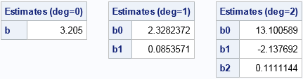
The output shows the parameter estimates for three regression models: a "mean model" (degree 0), a linear model (degree 1), and a quadratic model (degree 2). Notice that the parameter estimates for the weighted linear regression are the same as estimates computed by PROC REG in the previous section.

Score the weighted regression models

The previous section describes how to use SAS/IML to compute parameter estimates of weighted regression models, and you can also use SAS/IML to score the regression models. The scoring does not require knowing the weight variable, only the parameter estimates. The following module uses Horner's method to evaluate a polynomial on a grid of points:

/* Score regression fit on column vector x */
start PolyRegScore(x, coef);
   p = nrow(coef);
   y = j(nrow(x), 1, coef[p]);            /* initialize to coef[p] */
   do j = p-1 to 1 by -1; 
      y = y # x + coef[j];
   end;
   return(y);
finish;

You can compute predicted values for each model on a grid of points. You can then write the predicted values to a SAS data set and combine the predicted values and the original data. Lastly, you can use the SERIES statement in PROG SGPLOT to overlay the three regression models on the original data:

t = T( do(min(x), max(x), (max(x)-min(x))/25) ); /* uniform grid in range(X) */ 
Yhat = j(nrow(t), 3);
do d = 0 to 2;
   b = PolyRegEst(Y, X, w, d);                 /* weighted regression model of degree d */
   Yhat[,d+1] = PolyRegScore(t, b);            /* score model on grid */
end;
 
Z = t || Yhat;                                 /* write three predicted curves to data set */
create RegFit from Z[c={"t" "Pred0" "Pred1" "Pred2"}];
append from Z;
QUIT;
 
data RegAll;                                   /* merge predicted curves with original data */
label w="Weight" Pred0="Weighted Mean" 
      Pred1="Weighted Linear Fit" Pred2="Weighted Quadratic Fit";
merge RegData RegFit;
run;
 
title "Weighted Regression Models";            /* overlay weighted regression curves and data */
proc sgplot data=RegAll;
scatter x=x y=y / filledoutlinedmarkers markerattrs=(size=12 symbol=CircleFilled)
                  colorresponse=w colormodel=TwoColorRamp;
series x=t  y=Pred0 / curvelabel;
series x=t  y=Pred1 / curvelabel;
series x=t  y=Pred2 / curvelabel;
xaxis grid; yaxis grid;
run;

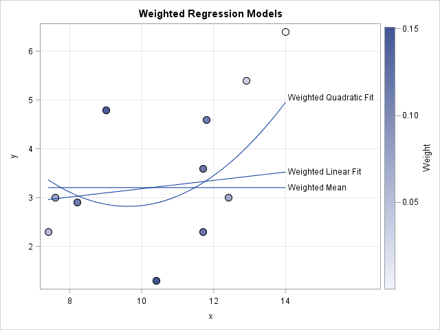
A visualization of the weighted regression models is shown to the left. The weighted linear fit is the same line that was shown in the earlier graph. The weighted mean and the weighted quadratic fit are the zero-degree and second-degree polynomial models, respectively. Of course, you could also create these curves in SAS by using PROC REG or by using the REG statement in PROC SGPLOT.

Summary

Weighted regression has many applications. The application featured in this article is to fit a model in which some response values are known with more precision than others. We saw that it is easy to create a weighted regression model in SAS by using PROC REG or PROC SGPLOT. It is only slightly harder to write a SAS/IML function to use matrix equations to "manually" compute the parameter estimates. No matter how you compute the model, observations that have relatively large weights are more influential in determining the parameter estimates than observations that have small weights.