Loess regression is a nonparametric technique that uses local weighted regression to fit a smooth curve through points in a scatter plot. Loess curves are can reveal trends and cycles in data that might be difficult to model with a parametric curve. Loess regression is one of several algorithms in SAS that can automatically choose a smoothing parameter that best fits the data.

In SAS, there are two ways to generate a loess curve. When you want to see statistical details for the fit, use the LOESS procedure. If you just want to overlay a smooth curve on a scatter plot, you can use the LOESS statement in PROC SGPLOT.

This article discusses the 1-D loess algorithm and shows how to control features of the loess regression by using PROC LOESS and PROC SGPLOT. You can also use PROC LOESS to fit higher dimensional data; the PROC LOESS documentation shows an example of 2-D loess, which fits a response surface as a function of two explanatory variables.

Overview of the loess regression algorithm

The loess algorithm, which was developed by Bill Cleveland and his colleagues in the late '70s through the 'early 90s, has had several different incarnations. Assume that you are fitting the loess model at a point x₀, which is not necessarily one of the data values. The following list describes the main steps in the loess algorithm as implemented in SAS:

1. Choose a smoothing parameter: The smoothing parameter, s, is a value in (0,1] that represents the proportion of observations to use for local regression. If there are n observations, then the k = floor(n*s) points closest to x₀ (in the X direction) form a local neighborhood near x₀.
2. Find the k nearest neighbors to x₀: I recently showed a SAS/IML module that can compute nearest neighbors.
3. Assign weights to the nearest neighbors: The loess algorithm uses a tricubic weight function to weight each point in the local neighborhood of x₀. The weight for the i_th point in the neighborhood is
   w_i = (32/5) (1- (d_i / D)³ )³
   where D is the largest distance in the neighborhood and d_i is the distance to the i_th point. (The weight function is zero outside of the local neighborhood.) The graph of the weight function is shown below: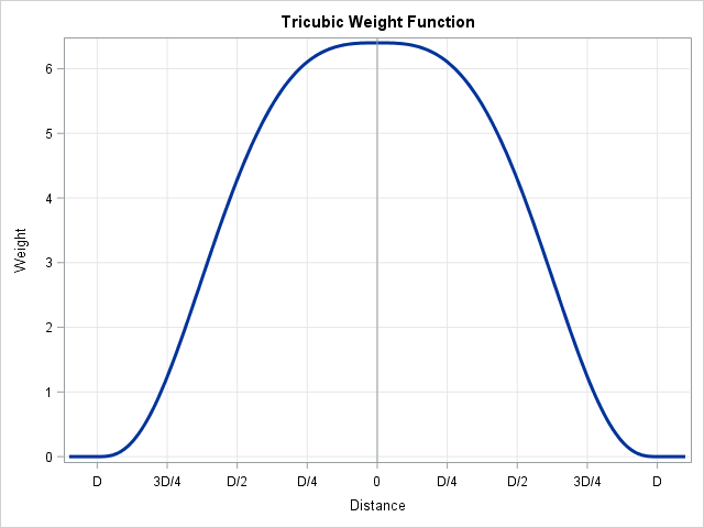
   The weight function gives more weight to observations whose X value is close to x₀ and less weight to observations that are farther away.
4. Perform local weighted regression: The points in the local neighborhood of x₀ are used to fit and score a local weighted regression model at x₀.

These four steps implement the basic loess method. The SAS procedures add a fifth step: optimize the smoothing parameter by fitting multiple loess models. You can use a criterion such as the AICC or GCV to balance the tradeoff between a tight fit and a complex model. For details, see the documentation for selecting the smoothing parameter.

How to score a loess regression model

The previous section told you how to fit a loess model at a particular point x₀. PROC LOESS provides two choices for the locations at which you can evaluate the model:

• By default, PROC LOESS evaluates the model at a data-dependent set of points, V, which are vertices of a k-d tree. Think of the points of V as a grid of X values. However, the grid is not linearly spaced in X, but is approximately linear in the quantiles of the data.
• You can evaluate the model at each unique X data value by using the DIRECT option on the MODEL statement.

If you want to score the model on a set of new observations, you cannot use the direct method. When you score new observations by using the SCORE statement, PROC LOESS uses linear or cubic interpolation between the points of V and the new observations. You can specify the interpolation scheme by using the INTERP= option on the MODEL statement.

Comparing PROC LOESS and the LOESS statement in PROC SGPLOT

The MODEL statement for the LOESS procedure provides many options for controlling the loess regression model. The LOESS statement in PROC SGPLOT provides only a few frequently used options. In some instances, PROC SGPLOT uses different default values, so it is worthwhile to compare the two statements.

• Choose a smoothing parameter: In both procedures, you can choose a smoothing parameter by using the SMOOTH= option.
• Fit the local weighted regression: In both procedures, you can control the degree of the local weighted polynomial regression by using the DEGREE= option. You can choose a linear or a quadratic regression model. Both procedures use the tricubic function to determine weights in the local neighborhood.
• Choose an optimal smoothing parameter: PROC LOESS provides the SELECT= option for controlling the selection of the optimal smoothing parameter. PROC SGPLOT does not provide a choice: it always optimizes the AICC criterion with the PRESEARCH suboption.
• Evaluate the fit: Both procedures evaluate the fit at a set of data-dependent values, then uses interpolation to evaluate the fit at other locations.
  • In PROC LOESS, you can use the SCORE statement to interpolate at an arbitrary set of points. You use the INTERP= option in the MODEL statement to specify whether to use linear or cubic interpolation.
  • In PROC SGPLOT, the interpolation is performed on a uniform grid of points. The default grid contains 201 points between min(x) and max(x), but you can use the MAXPOINTS= option to change that number. You use the INTERPOLATION= option to specify linear or cubic interpolation.

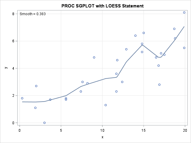
A loess example in SAS

The following SAS DATA step creates 30 observations for X and Y variables. The call to PROC LOESS creates a loess curve to the data and creates a fit plot, a residual plot, and a panel of diagnostic plots. Only the fit plot is shown:

data LoessData;
input x y @@;
datalines;
11.7  2.3  19.9  8.1  11.8  4.6  17.1  5.1  16.5  4.8
 5.6  1.7  12.9  5.4   7.6  3.0   9.0  4.8  17.5  5.0
10.4  1.3  16.9  2.8   5.6  1.8  18.7  6.9   3.7  1.7
 7.4  2.3   2.0  2.7  14.8  5.2   3.0  0.0  16.8  4.2
15.0  6.6  19.9  5.5   1.9  1.1  14.8  5.8  12.4  3.0
14.0  6.4  11.7  3.6   8.2  2.9  18.8  6.2   0.3  1.8
;
 
ods graphics on;
ods select FitPlot;
proc loess data=LoessData plots=FitPlot;
model y = x / interp=linear           /* LINEAR or CUBIC */
              degree=1                /* 1 or 2 */
              select=AICC(presearch); /* or SMOOTH=0.383 */
run;

For the PROC LOESS call, all options are the default values except for the PRESEARCH suboption in the SELECT= option. You can create the same fit plot by using the LOESS statement in PROC SGPLOT. The default interpolation scheme in PROC SGPLOT is cubic, so the following statements override that default option:

title "PROC SGPLOT with LOESS Statement";
proc sgplot data=LoessData  noautolegend;
loess x=x y=y / interpolation=linear  /* CUBIC or LINEAR */
                degree=1              /* 1 or 2 */
                ;  /* default selection or specify SMOOTH=0.383 */
xaxis grid; yaxis grid;
run;

The two plots are shown side by side. The one on the left was created by PROC LOESS. The one on the right was created by PROC SGPLOT.

In conclusion, SAS provides two ways to overlay a smooth loess curve on a scatter plot. You can use PROC LOESS when you want to see the details of statistical aspects of the fit and the process that optimizes the smoothing parameter. You can use the SGPLOT procedure when you care less about the details, but simply want an easy way to show a nonlinear relationship between a response and an explanatory variable.