A previous post discusses how the loess regression algorithm is implemented in SAS. The LOESS procedure in SAS/STAT software provides the data analyst with options to control the loess algorithm and fit nonparametric smoothing curves through points in a scatter plot.

Although PROC LOESS satisfies 99.99% of SAS users who want to fit a loess model, some research statisticians might want to extend or modify the standard loess algorithm. Researchers like to ask "what if" questions like "what if I used a different weighting function?" or "what if I change the points at which the loess model is evaluated?" Although the loess algorithm is complicated, it is not hard to implement a basic version in a matrix language like SAS/IML.

Implement loess regression in SAS/IML

Recent blog posts have provided some computational modules that you can use to implement loess regression. For example, the PairwiseNearestNbr module finds the k nearest neighbors to a set of evaluation points. The functions for weighted polynomial regression computes the loess fit at a particular point.

You can download a SAS/IML program that defines the nearest-neighbor and weighted-regression modules. The following call to PROC IML loads the modules and defines a function that fits a loess curve at points in a vector, t. Each fit uses a local neighborhood that contains k data values. The local weighted regression is a degree-d polynomial:

proc iml;
load  module=(PairwiseNearestNbr PolyRegEst PolyRegScore);
/* 1-D loess algorithm. Does not handle missing values.
   Input: t: points at which to fit loess (column vector)
          x, y: nonmissing data (column vectors)
          k: number of nearest neighbors used for loess fit
          d: degree of local regression model 
   Output: column vector L[i] = f(t[i]; k, d) where f is loess model
*/
start LoessFit(t, x, y, k, d=1);
   m = nrow(t);
   Fit = j(m, 1);                            /* Fit[i] is predicted value at t[i] */
   do i = 1 to m;
      x0 = t[i];
      run PairwiseNearestNbr(idx, dist, x0, x, k);
      XNbrs = X[idx];  YNbrs = Y[idx];       /* X and Y values of k nearest nbrs */
      /* local weight function where dist[,k] is max dist in neighborhood */
      w = 32/5 * (1 - (dist / dist[k])##3 )##3; /* use tricubic weight function */
      b = PolyRegEst(YNbrs, XNbrs, w`, d);   /* param est for local weighted regression */
      Fit[i] = PolyRegScore(x0, b);          /* evaluate polynomial at x0 */
   end;
   return Fit;
finish;

This algorithm provides some features that are not in PROC LOESS. You can use this function to evaluate a loess fit at arbitrary X values, whereas PROC LOESS evaluates the function only at quantiles of the data. You can use this function to fit a local polynomial regression of any degree (for example, a zero-degree polynomial), whereas PROC LOESS fits only first- and second-degree polynomials. Although I hard-coded the standard tricubic weight function, you could replace the function with any other weight function.

On the other hand, PROC LOESS supports many features that are not in this proof-of-concept function, such as automatic selection of the smoothing parameter, handling missing values, and support for higher-dimensional loess fits.

Call the loess function on example data

Let's use polynomials of degree 0, 1, and 2 to compute three different loess fits. The LoessData data set is defined in my previous article:

use LoessData;  read all var {x y};  close;   /* read example data */
 
s = 0.383;                /* specify smoothing parameter */
k = floor(nrow(x)*0.383); /* num points in local neighborhood */
 
/* grid of points to evaluate loess curve (column vector) */
t    = T( do(min(x), max(x), (max(x)-min(x))/50) );
Fit0 = LoessFit(t, x, y, k, 0);    /* loess fit with degree=0 polynomials */
Fit1 = LoessFit(t, x, y, k, 1);    /* degree=1 */
Fit2 = LoessFit(t, x, y, k, 2);    /* degree=2 */
 
create Sim var {x y t Fit0 Fit1 Fit2};  append;  close;
QUIT;

You can use PROC SGPLOT to overlay these loess curves on a scatter plot of the data:

title "Overlay loess curves computed in SAS/IML";
proc sgplot data=Sim;
label Fit0="Loess (Deg=0)" Fit1="Loess (Deg=1)" Fit2="Loess (Deg=2)"; 
scatter x=x y=y;
series x=t  y=Fit0 / curvelabel;
series x=t  y=Fit1 / curvelabel lineattrs=(color=red);
series x=t  y=Fit2 / curvelabel lineattrs=(color=ForestGreen);
xaxis grid; yaxis grid;
run;

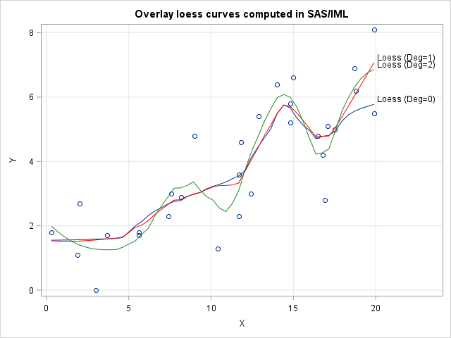
The three curves are fairly close to each other on the interior of the data. The degree 2 curve wiggles more than the other two curves because it uses a higher-degree polynomial. The over- and undershooting becomes even more pronounced if you use cubic or quartic polynomials for the local weighted regressions.

The curious reader might wonder how these curves compare to curves that are created by PROC LOESS or by the LOESS statement in PROC SGPLOT. In the attached program I show that the IML implementation produces the same predicted values as PROC LOESS when you evaluate the models at the same set of points.

Most SAS data analysts are happy to use PROC LOESS. They don't need to write their own loess algorithm in PROC IML. However, this article shows that IML provides the computational tools and matrix computations that you need to implement sophisticated algorithms, should the need ever arise.