If you perform a weighted statistical analysis, it can be useful to produce a statistical graph that also incorporates the weights. This article shows how to construct and interpret a weighted histogram in SAS.

How to construct a weighted histogram

Before constructing a weighted histogram, let's review the construction of an unweighted histogram. A histogram requires that you specify a set of evenly spaced bins that cover the range of the data. An unweighted histogram of frequencies is constructed by counting the number of observations that are in each bin. Because counts are dependent on the sample size, n, histograms often display the proportion (or percentage) of values in each bin. The proportions are the counts divided by n. On the proportion scale, the height of each bin is the sum of the quantity 1/n, where the sum is taken over all observations in the bin.

That fact is important because it reveals that the unweighted histogram is a special case of the weighted histogram. An unweighted histogram is equivalent to a weighted histogram in which each observation receives a unit weight. Therefore the quantity 1/n is the standardized weight of each observation: the weight divided by the sum of the weights. The formula is the same for non-unit weights: the height of each bin is the sum of the quantity w_i / Σ w_i, where the sum is taken over all observations in the bin. That is, you add up all the standardized weights in each bin to produce the bin height.

An example of a weighted histogram

The SAS documentation for the WEIGHT statement includes the following example. Twenty subjects estimate the diameter of an object that is 30 cm across. Some people are placed closer to the object than others. The researcher believes that the precision of the estimate is inversely proportional to the distance from the object. Therefore the researcher weights each subject's estimate by using the inverse distance.

The following DATA step creates the data, and PROC SGPLOT creates a weighted histogram of the data by using the WEIGHT= option on the HISTOGRAM option. (The WEIGHT= option was added in SAS 9.4M1.)

data Size;
input Distance ObjectSize @@;
Wt = 1 / distance;        /* precision */
x = ObjectSize; 
label x = "Estimate of Size";
datalines;
1.5 30   1.5 20   1.5 30   1.5 25
3   43   3   33   3   25   3   30
4.5 25   4.5 36   4.5 48   4.5 33
6   43   6   36   6   23   6   48
7.5 30   7.5 25   7.5 50   7.5 38
;
 
title "Weighted Histogram of Size Estimate";
proc sgplot data=size noautolegend;
   histogram x / WEIGHT=Wt scale=proportion datalabel binwidth=5;
   fringe x / lineattrs=(thickness=2 color=black) transparency=0.6;
   yaxis grid offsetmin=0.05 label="Weighted Proportion";
   refline 30 / axis=x lineattrs=(pattern=dash);
run;

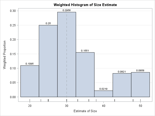
The weighted histogram is shown to the right. The data values are shown in the fringe plot beneath the histogram. The height of each bin is the sum of the weights of the observations in that bin. The dashed line represents the true diameter of the object. Most estimates are clustered around the true value, except for a small cluster of larger estimates. Notice that I use the SCALE=PROPORTION option to plot the weighted proportion of observations in each bin, although the default behavior (SCALE=PERCENT) would also be acceptable.

If you remove the WEIGHT= option and study the unweighted graph, you will see that the average estimate for the unweighted distribution (33.6) is not as close to the true diameter as the weighted estimate (30.1). Furthermore, the weighted standard deviation is about half the unweighted standard deviation, which shows that the weighted distribution of these data has less variance than the unweighted distribution.

By the way, although PROC UNIVARIATE can produce weighted statistics, it does not create weighted graphics as of SAS 9.4M5. One reason is that the graphics statements (CDFPLOT, HISTOGRAM, QQPLOT, etc) not only create graphs but also fit distributions and produce goodness-of-fit statistics, and those analyses do not support weight variables.

Checking the computation

Although a weighted histogram is not conceptually complex, I understand a computation better when I program it myself. You can write a SAS program that computes a weighted histogram by using the following algorithm:

1. Construct the bins. For this example, there are eight bins of width 5, and the first bin starts at x=17.5. (It is centered at x=20.) Initialize all bin heights to zero.
2. For each observation, find the bin that contains it. Increment the bin height by the weight of that observation.
3. Standardize the heights by dividing by the sum of weights. You can skip this step if the weights sum to unity.

A SAS/IML implementation of this algorithm requires only a few lines of code. A DATA step implementation that uses arrays is longer, but probably looks more familiar to many SAS programmers:

data BinHeights(keep=height:);
array EndPt[8] _temporary_;
binStart = 17.5;  binWidth = 5;  /* anchor and width for bins */
do i = 1 to dim(EndPt);          /* define endpoints of bins */
   EndPt[i] = binStart + (i-1)*binWidth;
end;
 
array height[7];                 /* height of each bin */
set Size end=eof;                /* for each observation ... */
sumWt + Wt;                      /* compute sum of weights */
Found=0;
do i = 1 to dim(EndPt)-1 while (^Found); /* find bin for each obs */
   Found = (EndPt[i] <= x < EndPt[i+1]);
   if Found then height[i] + Wt; /* increment bin height by weight */
end;
if eof then do;            
   do i = 1 to dim(height);      /* scale heights by sum of weights */
      height[i] = height[i] / sumWt;
   end;
   output;
end;
run;
 
proc print noobs data=BinHeights; run;

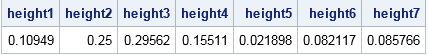
The computations from the DATA step match the data labels that appear on the weighted histogram in PROC SGPLOT.

Summary

In SAS, the HISTOGRAM statement in PROC SGPLOT supports the WEIGHT= option, which enables you to create a weighted histogram. A weighted histogram shows the weighted distribution of the data. If the histogram displays proportions (rather than raw counts), then the heights of the bars are the sum of the standardized weights of the observations within each bin. You can download the SAS program that computes the quantities in this article.

How can you interpret a weighted histogram? That depends on the meaning of the weight variables. For survey data and sampling weights, the weighted histogram estimates the distribution of a quantity in the population. For inverse variance weights (such as were used in this article), the weighted histogram overweights precise measurements and underweights imprecise measurements. When the weights are correct, the weighted histogram is a better estimate of the density of the underlying population and the weighted statistics (mean, variance, quantiles,...) are better estimates of the corresponding population quantities.

Have you ever plotted a weighted histogram? What was the context? Leave a comment.