When you are working with probability distributions (normal, Poisson, exponential, and so forth), there are four essential functions that a statistical programmer needs. As I've written before, for common univariate distributions, SAS provides the following functions:
- the PDF function, which returns the probability density at a given point
- the CDF function, which returns the probability that an observation from the specified distribution is less than or equal to a particular value
- the QUANTILE function, sometimes called the inverse CDF function
- the RAND function, which generates a random sample from a distribution. (In SAS/IML software, use the RANDGEN subroutine, which fills up an entire matrix at once.)
Evaluating the multivariate versions of these functions is harder. As I showed last week, you can define the multivariate PDF function by using the SAS/IML language. SAS/IML software also provides several built-in functions for simulating random variates from various useful multivariate distributions, and my forthcoming book describes how to simulate data from additional distributions.
However, the multivariate CDF function is hard to compute because it requires high-dimensional numerical integration of complicated functions. (I'll ignore the trivial distributions, such as the multivaraite uniform distribution.) The multivariate quantile function is also difficult to compute, in part because it requires the multivariate CDF, but also because a quantile of a multivariate distribution is not a single point. For bivariate distributions, a quantile is usually a curve, and, in general, for a multivariate distribution with n variables a quantile is an (n-1)-dimensional isosurface.
However, for the bivariate normal distribution, SAS provides a function that accurately performs the numerical integration that is needed to compute the bivariate normal CDF: the PROBBNRM function.
Don't use the PROB* functions! (Except two)
I used SAS for many years before I learned about the PROBBNRM function. Why? Because when I look at the documentation for SAS functions, I've trained my eyes to skip over all of the functions that begin with "PROB" because these functions are replaced by the newer CDF function, which can compute the CDF for many univariate distributions.
Then one day I saw a reference to the PROBBNRM function in a journal article. I looked it up in the SAS documentation and have used it ever since!
Oh, and the PROBMC function is also useful. I've used it to compute decision limits for multiple comparisons.
Evaluating the bivariate normal CDF
The PROBBNRM function returns the probability that an observation (x, y) from a standardized bivariate normal distribution with mean 0, variance 1, and correlation coefficient r, is less than or equal to (x, y). Geometrically, the bivariate normal CDF at the point (x1,x2) is the volume under the graph of the bivariate normal PDF on the domain [-∞, x]×[-∞,y]. Using the symmetries of the standardized bivariate normal PDF, a few facts are obvious:
- For uncorrelated variables, the volume under the density surface for the lower left quadrant of the plane is 1/4. This means that PROBBNRM(0,0,0) is 1/4.
- For any standardized distribution the volume under the density surface for the left half-plane is 1/2. This means that PROBBNRM(0,b,r) is approximately 1/2 when b is sufficiently large.
- Similarly, PROBBNRM(a,0,r) is approximately 1/2 when a is sufficintly large.
- Because the total volume under the surface is 1, PROBBNRM(a, b,r) is approximately 1 when a and b are sufficiently large.
The following SAS/IML statements test these facts, as a way of making sure that PRBBNRM function behaves like we expect:
proc iml;
x = {0 0,
     5 0,
     0 5,
     5 5};
r = 0;         /* uncorrelated vars */
p0 = probbnrm(x[,1],x[,2],r);
r = sqrt(2)/2; /* correlated vars */
p1 = probbnrm(x[,1],x[,2],r);
print p0 p1; |
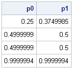
The limiting cases are as expected. So what does the graph of the bivariate CDF look like over, say, [-3,3]×[-3,3]? Well, the CDF is essentially zero near (-3,-3) and essentially 1 near (3,3). If you fix any value x=x0, the function is monotone increasing as a function of y. By symmetry, the same holds if you reverse the roles of x and y. To visualize the function, you can use the same steps that I used to visualize the bivariate normal PDF:
x = ExpandGrid( do(-3, 3, 0.1), do(-3, 3, 0.1) );
rho = sqrt(2)/2; /* correlation */
cdf = probbnrm(x[,1], x[,2], rho);

x1 = x[,1]; x2 = x[,2];
create BivarCDF var {"x1" "x2" "CDF"};
append;
close BivarCDF;

proc sgrender data=BivarCDF template=ContourPlotParm;
dynamic _TITLE="Bivariate Normal CDF, corr=sqrt(2)/2"
        _X="x1" _Y="x2" _Z="CDF";
run; |
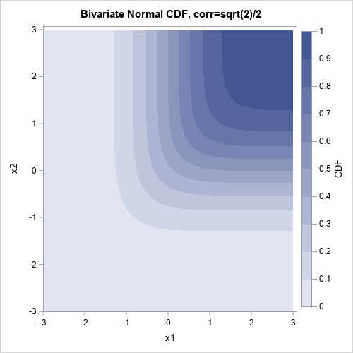
The contour plot of the bivariate normal CDF also shows quantiles of the CDF. By definition, the quantiles for α are the set of points for which CDF(x1,x2) = α. These are exactly the contours of the CDF function.

7 Comments
Then what is the difference between the PROB* functions and the CDF functions? Do they have the same results?
The PROB* functions are the old function that compute probabilities, just like the RAN* functions (RANUNI, RANNOR, RANGAM, etc) are the old functions for generating random variates and the *INV functions (GAMINV, BETAINV, etc) are the old quantile functions.
Use the newer CDF, PDF, RAND, and QUANTILE functions. The newer functions use the latest algorithms and can compute results in the tails of distributions that might trip up the older routines. For typical ranges of the parameters, you might not see any differences, but for extreme values I recommend the newer functions.
Great! Thanks a lot for this detailed answer.
Pingback: The gradient of the bivariate normal cumulative distribution - The DO Loop
Pingback: Compute contours of the bivariate normal CDF - The DO Loop
Pingback: Monte Carlo estimates of joint probabilities - The DO Loop
Pingback: Bivariate normal probability in SAS: Rectangular regions - The DO Loop