I've been working on a new book about Simulating Data with SAS. In researching the chapter on simulation of multivariate data, I've noticed that the probability density function (PDF) of multivariate distributions is often specified in a matrix form. Consequently, the multivariate density can usually be computed by using the SAS/IML matrix language. As an example, this article describes how to compute the multivariate normal probability density for an arbitrary number of variables.
Compute the multivariate normal PDF
The density for the multivariate distribution centered at μ with covariance Σ is given by the following formula, which I copied from a Wikipedia article:

The argument to the EXP function involves the expression d2=(x-μ)TΣ-1(x-μ), where d is the Mahalanobis distance between the multidimensional point x and the mean vector μ. I have previous written a SAS/IML function that computes the Mahalanobis distance in SAS, so it is simple to construct a SAS/IML function that computes the multivariate normal PDF for any dimension:
proc iml;
/* Cut and paste the definition of the Mahalanobis module. See
https://blogs.sas.com/content/iml/2012/02/22/how-to-compute-mahalanobis-distance-in-sas/ */
start MVNormalPDF(x, mu, cov);
   p = nrow(cov);
   const = (2*constant("PI"))##(p/2) * sqrt(det(cov));
   d = Mahalanobis(x, mu, cov);
   phi = exp( -0.5*d#d ) / const;
   return( phi );
finish; |
The MVNormalPDF function is essentially an implementation of the PDF formula, except that the (efficient) Mahalanobis function is used instead of explicitly forming the expression (x-μ)TΣ-1(x-μ). Incidentally, the formula assumes that x and μ are a column vectors. However, the Mahalanobis and MVNormalPDF functions assume that mu is a row vector, and evaluates the PDF on each row of the x matrix.
Evaluating the multivariate normal PDF
Although it is not apparent at first glance, the MVNormalPDF function is vectorized, which means that the x argument can be an N x p matrix that represents N different p-dimensional points. The vectorization results from the fact that the Mahalanobis function is vectorized.
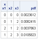
This means that you can evaluate the PDF at many points by using a single call, as shown below for a three-dimensional example:
Mu  = {1 2 3};
Cov = {3 2 1,
       2 4 0,
       1 0 5};
x = {0 0 0,
     0 1 2,
     2 1 2,
     1 2 3};
pdf = MVNormalPDF(x, Mu, Cov);
print x[c=("x1":"x3")] pdf; |
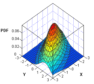
Visualize the bivariate normal PDF
In the case of two variables, you can visualize the bivariate normal density by creating a surface plot or contour plot. In either case, you need to evaluate the MVNormalPDF function at a grid of (x,y) values. You can use the Define2DGrid function to generate evenly spaced (x,y) values on a uniform grid. The following SAS/IML statements load the Define2DGrid function, evaluate the bivariate normal density at a grid of points, and write the data to a SAS data set:
/* define or load Define2DGrid module:
https://blogs.sas.com/content/iml/2011/01/21/how-to-create-a-grid-of-values/ */
load module=Define2DGrid;
Mu = {0 0};
Cov = {4 2, /* correlation coefficient is sqrt(2) */
       2 2};
x = Define2DGrid( -3, 3, 31, -3, 3, 31 ); /* grid is [-3,3]x[-3,3] */
density = MVNormalPDF(x, Mu, Cov);

x1 = x[,1]; x2 = x[,2];
create BivarDensity var {"x1" "x2" "Density"};
append;
close BivarDensity;
quit; |
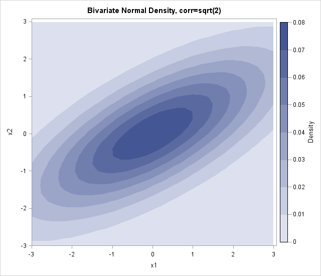
Earlier this week, I showed how to create a contour plot in SAS by using the Graph Template Language (GTL). Assuming that the ContourPlotParm template has been defined, the following call to the SGRENDER procedure creates a contour plot of the bivariate normal data:
proc sgrender data=BivarDensity template=ContourPlotParm; dynamic _TITLE="Bivariate Normal Density, corr=sqrt(2) " _X="x1" _Y="x2" _Z="Density"; run; |

17 Comments
Can we calculate Multivariate Normal Density in base SAS without using IML as I dont have access to it.
Wikipedia has a formula for the bivariate density that you can program in the DATA step. You can do an internet search for "trivariate normal density" to find the formula for three variables.
Pingback: Visualize the bivariate normal cumulative distribution - The DO Loop
Rick,
Thank you indeed for your answer. I simply tried to replicate your results with the program you posted.
proc iml;
/* define or load Mahalanobis module:
http://blogs.sas.com/content/iml/2012/02/22/how-to-compute-mahalanobis-distance-in-sas/ */
load module=Mahalanobis;
start MVNormlPDF(x, mu, cov);
p = nrow(cov);
const = (2*constant("PI"))##(p/2) * sqrt(det(cov));
d = Mahalanobis(x, mu, cov);
phi = exp( -0.5*d#d ) / const;
return( phi );
finish;
Mu = {1 2 3};
Cov = {3 2 1,
2 4 0,
1 0 5};
x = {0 0 0,
0 1 2,
2 1 2,
1 2 3};
pdf = MVNormalPDF(x, Mu, Cov);
print x[c=("x1":"x3")] pdf;
run;
but in the log window, unfortunately i am getting the same error as i had before.
ERROR: Unable to load module MAHALANOBIS. [Entry MAHALANOBIS.IMOD not found in catalog WORK.IMLSTOR.]
though Module MVNORMLPDF defined.
i do not know that wrong is with the program or not able to load the module. Thanks.
Sorry for your confusion. Notice that the comment links to an article in which I define the Mahalanobis module. Go to that URL and paste in the definition of the Mahalanobis function. I have rewritten the comment to make it more clear.
Rick,
proc iml;
start MVNormalPDF(x, mu, cov);
y = (x-mu)
* inv(cov) * y;
p = nrow(cov);
const = (2*constant("PI"))##(p/2) * sqrt(det(cov));
phi = exp( -0.5*d#d ) / const;
return( phi );
finish;
Mu = {1 2 3};
Cov = {3 2 1,
2 4 0,
1 0 5};
x = {0 0 0,
0 1 2,
2 1 2,
1 2 3};
pdf = MVNormalPDF(x, Mu, Cov);
print x[c=("x1":"x3")] pdf;
this program works and produces pdf at each x.
Also, in your post, there is a word error between MVNormlPDF in "start" function and pdf = MVNormalPDF(x, Mu, Cov). Thanks a lot.
Yes, you can do that. That technique is inefficient for large dimenions, which I point out at http://blogs.sas.com/content/iml/2012/02/22/how-to-compute-mahalanobis-distance-in-sas/. My intention was for you to cut and paste the Mahalanobis function from that URL. However, for small dimensions, your technique is fine and is simpler.
Thanks for catching the typo. It is fixed.
Dear Dr Wicklin,
It works perfect. Thanks a lot.
Pingback: Compute a contour (level curve) in SAS - The DO Loop
Pingback: How to generate a grid of points in SAS - The DO Loop
Dear Rick,
I tried the corrected code given by Abdulbaki Bilgic. But still it shows error "Matrices do not conform to the operation". I followed your other post as well on the error part but still it is not resolved. Please help me with the code. I have gone through your other posts as well and they are very intuitive and very helpful.
Regards,
Varun
Whenever you have questions about SAS/IML programming, you can post your question (along with your program and data) to the SAS/IML Support Community.
Can we calculate Multivariate Normal CDF in SAS?
You can use the PROBBNRM function to compute the bivariate normal CDF. For higher dimensions, there have been some discussions on the SAS Support Communities. One discusses the Monte Carlo approach for t distributions, but also applies to MVN distributions.
Thank you for your prompt reply.I will go to this link to learn about it.
I need to estimate the parameters of a set of bivariate gaussians from data. The data take the form of an n x n identification/confusion matrix where n is the the number of response alternatives. In its most basic form, the stimuli are formed from two dimensions (e.g., height, width), with two levels of each dimension, giving four response alternatives. It is also assumed that there is a decision bound for each dimension, giving a total of a mean vector and covariance matrix for each response alternative, and two decision bounds. Could this code be adapted to this problem, and if so, what would your recommendation be for proceeding. My thanks in advance!
Pingback: Compute the multivariate t density function - The DO Loop