I recently posted an article about representing uncertainty in rankings on the blog of the ASA Section for Statistical Programmers and Analysts (SSPA). The posting discusses the importance of including confidence intervals or other indicators of uncertainty when you display rankings.
Today's article complements the SSPA post by showing how to construct the confidence intervals in SAS. This article implements the techniques in Marshall and Spiegelhalter (1998), Brit. Med. J., which is a very well written and readable paper. (If you prefer sports to medicine, Spiegelhalter wrote a similar article on ranking teams in the English Premier Football League.)
To illustrate the ideas, consider the problem of ranking US airlines on the basis of their average on-time performance. The data for this example are described in the Statistical Computing and Graphics Newsletter (Dec. 2009) and in my 2010 SAS Global Forum paper. The data are available for download.
The data are in a SAS data set named MVTS that consists of 365 observations and 21 variables. The Date variable records the day in 2007 for which the data were recorded. The other 20 variables contain the mean delays, in minutes, experienced by an airline carrier for that day's flights. The airline variables in the data are named by using two-digit airline carrier codes. For example, AA is the carrier code for American Airlines.
The appendix of Marshall and Spiegelhalter's paper describes how to compute rankings with confidence intervals:
- Compute the mean delay for each airline in 2007.
- Compute the standard error for each mean.
- Use a simulation to compute the confidence intervals for the ranking.
Ordering Airlines by Mean Delays
You can use PROC MEANS or PROC IML to compute the means and standard errors for each carrier. Because simulation will be used in Step 3 to compute confidence intervals for the rankings, PROC IML is the natural choice for this analysis. The following statements compute the mean delay for all airlines (sometimes called the "grand mean") and the mean delays for each airline in 2007. The airlines are then sorted by their mean delays, as described in a previous article about ordering the columns of a matrix.
proc iml;
/** read mean delay for each day in 2007
    for each airline carrier **/
Carrier = {AA AQ AS B6 CO DL EV F9 FL HA
           MQ NW OH OO PE UA US WN XE YV};
use dir.mvts;
read all var Carrier into x;
close dir.mvts;

grandMean = x[:];
meanDelay = x[:,];
call sortndx(idx, MeanDelay`, 1);

/** reorder columns **/
Carrier = Carrier[,idx];
x = x[,idx];
meanDelay = meanDelay[,idx];
print grandMean, carrier;

------- OUTPUT ---------
               grandMean

               9.6459671


                Carrier

AQ HA WN DL F9 FL PE OO AS XE CO YV ... AA EV |
You can use these computations to reorder the variables in the data set (this step is not shown) and use PROC SGPLOT to plot the means and standard errors for the each airline carrier:
/** convert data from wide to long format**/ proc transpose data=mvts out=Delay(rename=(col1=Delay)) name=Carrier; by date; run; title "Comparison of Airline Daily Delays (2007)"; proc sgplot data=delay noautolegend; dot carrier / response=delay stat=mean limitstat=clm; refline 9.646 / axis=x lineattrs=(pattern=dash); xaxis label="Mean Delay with 95% Confidence Intervals"; yaxis discreteorder=data label="Carrier"; run; |
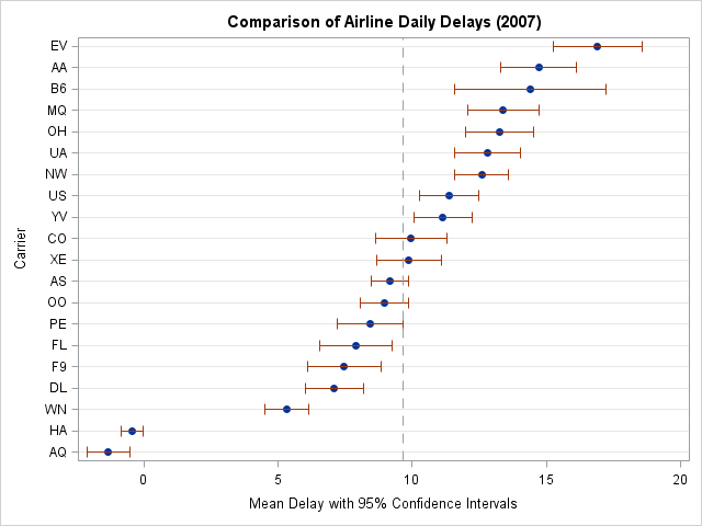
Notice that two airlines (Aloha Airlines (AQ) and Hawaiian Airlines (HA)) have much better on-time performance than the others. In fact, their average daily delay is negative, which means that they typically land a minute or two ahead of schedule!
Many analysts would end the analysis here by assigning ranks based on the mean statistics. But as I point out on my SSPA blog, it is important for rankings to reflect the uncertainty in the mean estimates.
Notice that for most airlines, the confidence interval overlaps with the confidence intervals of one or more other airlines. The "true mean" for each airline is unknown but probably lies within the confidence intervals.
So, for example, Frontier Airlines (F9) is nominally ranked #5. But you can see from the overlapping confidence intervals that there is a chance that the true mean for Frontier Airlines is lower than the true mean of Delta Airlines (DL), which would make Frontier ranked #4. However, there is also a chance that the true mean could be less than the true mean of Continental Airlines (CO), which would make Frontier ranked #11. How can you rank the airlines so that that uncertainty is reflected in the ranking?
The answer is in Step 3 of Marshall and Spiegelhalter's approach: use a simulation to compute the confidence intervals for the ranking. This step will appear in a second article, which I will post next week.

4 Comments
Pingback: Ranking with confidence: Part 2 - The DO Loop
Pingback: Funnel plots: An alternative to ranking - The DO Loop
Pingback: Creating bar charts with confidence intervals - The DO Loop
Pingback: Readers’ choice 2011: The DO Loop’s 10 most popular posts - The DO Loop