An NMF analysis of Scotch whiskies

This is the last article in a series about the nonnegative matrix factorization (NMF). In this article, I run and visualize an NMF analysis of the Scotch whisky data and compare it to a principal component analysis (PCA).

Previous articles in the series provide information about the whisky data, the PCA analysis, and issues related to two-factor low-rank factorizations such as the NMF:

PCA Analysis of whisky: What is the Scotch whisky data? How can you use a PCA to identify whiskies that have similar flavor characteristics?
A two-factor rank-k decomposition has inherent ambiguities: You can arbitrarily scale and permute the order of the factors.
A comparison of the PCA and NMF decompositions on simulated data, which reveals why the NMF might be preferred for nonnegative data.

In SAS, you can obtain the NMF by using PROC NMF in SAS Viya, or by implementing the algorithm directly in SAS IML. Sharad Saxena has written three blog posts about how to use PROC NMF in SAS Viya:

Dimension reduction by using the NMF

A previous article uses classical principal component analysis (PCA) to analyze the flavor profiles of 86 Scotch whiskies. Each whisky is assigned a value 0-4 according to 12 flavors: Tobacco, Medicinal, Smoky, Body, Spicy, Winey, Nutty, Honey, Malty, Fruity, Sweetness, and Floral. The PCA and NMF analyses were discussed in an article by Young, Fogel, and Hawkins (2006, "Clustering scotch whiskies using non-negative matrix factorization", SPES Newsletter).

By using the PCA, you can find a low-dimensional linear subspace in the 12-dimensional variable space such that the subspace captures most of the variance in the data. This is called dimension reduction. For the whisky data, you can use PCA to choose a four-dimensional subspace that explains 67% of the variability in the data. The PCA factorization has two important properties: it maximizes the explained variance of the data within a lower-dimensional linear subspace, and it provides orthogonal basis vectors for the subspace.

Whereas the PCA can analyze any centered data matrix, the NMF factorization is designed for dimension-reduction of a nonnegative data matrix. The NMF seeks to decompose the data matrix into profile vectors (which are basis vectors for a lower-dimensional subspace) and a matrix of weights so that the product approximates the data matrix. In addition, the NMF requires that the profile vectors and weights be nonnegative. This last condition is why the NMF factors are often more interpretable than the PC vectors. However, the NMF decomposition does not have the maximum-variance or orthogonal-basis properties that make the PCA useful.

How to interpret the NMF factors

The whisky data can be represented as an 86x12 nonnegative data matrix, X. Each row represents flavor characteristics of a whisky. Each whisky is assigned a flavor profile that consists of the values 0-4 for the 12 flavors.

The NMF creates a rank-4 approximation to X. The approximation is represented as a product W*H, where W is 86x4 and H is 4x12. The rows of H form a basis for a 4-D linear subspace. These are the "flavor profile" vectors that are analogous to the principal components (eigenvectors) in a PCA analysis.

The rows of the W matrix are weights (or coefficients) for the 4-factor approximation of X. If W_i is the i_th row of W, the product W_i * H approximates the flavor profile for the i_th whisky. Equivalently, if H₁-H₄ are the rows of H, then the linear combination
W_i1H₁ + W_i2H₂ + W_i3H₃ + W_i4H₄
is an approximation of the flavors for the i_th whisky. In this sense, W provides the weights for the approximation in terms of the NMF profile vectors.

Be aware that the role played by W and H depends on how the data are arranged in X. For example, it is equally valid to represent the data by using a 12x86 data matrix, Y, where the rows are the flavors and the columns are the whiskies. In that case, Y` = X, and Y = H`*W` is a valid NMF factorization.

An NMF analysis of the whisky data

I'm a statistician, not a Scotch connoisseur. Nevertheless, let's perform an NMF analysis of the whisky data. I used SAS IML to implement a simple version of the NMF algorithm. You can download the SAS programs in this article from GitHub and run the analysis yourself. After reading the whisky data into a matrix, the following IML statements perform an NMF analysis and visualize the H matrix. Since the rows of H are the basis vectors for a 4-D subspace, I transpose the matrix and display the columns. As shown in a previous article, you can scale the NMF factors so that they are approximately on the same scale as the PCA factors.

%let varNames = Tobacco Medicinal Smoky Body Spicy Winey Nutty Honey Malty Fruity Sweetness Floral;
proc iml;
/* Apply NMF to the Scotch whisky data */
varNames = propcase({&varNames});
use Whisky;
   read all var varNames into X;
   read all var {"Distillery" "Selected"};
close;
 
/* The PCA analysis of the whisky data kept four PCs.
   Load the nmf_mult function and compute a four-factor NMF */
load module = _ALL_;
names = 'NMF 1':'NMF 4';
run nmf_mult(W1, H1, X, ncol(names));
 
/* scale the H matrix to use the same scale used in the PCA article */
maxValPCA = 0.8506;             /* max value in the PCA eigenbasis */
scale = maxValPCA / H1[,<>];    /* scale each row by maximum, then multiply by maxVal */
W = W1 / scale`;
H = H1 # scale;
print  (W[<>,])[L="Max W Cols"],   (H[,<>])[L="Max H Rows"];
 
%let Reds = CXF7F7F7 CXFDDBC7 CXF4A582 CXD6604D CXB2182B ;
ods graphics / width=360px height=480px;
call heatmapcont(H`) title="NMF Factors (H`) for Whiskies"
                     colorramp={&Reds} range=(0||max(H))
                     xvalues=names yvalues=varNames;

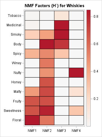
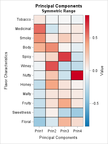
For comparison, I also show a heat map of the factors (basis elements) for the four-component PCA analysis from my previous article. The colors in the left image correspond to the interval [0, 0.8506]. The colors in the right image correspond to the interval [-0.8506, 0.8506], where white represents 0, so that the red colors represent the same range in each image. The images enable you to compare the NMF and PCA factors. Here are some comparisons:

Both images show latent factors for a four-factor approximation of the whisky flavors. That is, the flavor characteristics of all whiskies are approximated by linear combinations of these four factors.
The factors for the NMF are all positive. Because the weights are also positive, the flavor of each whisky is approximated by using an additive sum of these NMF components. In contrast, the PCA factors have both positive and negative values. The flavor of each whisky is approximated by using a sum of these contrasts.
The first NMF factor is a strong combination of the Fruity, Sweetness, and Floral variables, with smaller amounts of Smoky, Spicy, and Malty. At the risk of promoting stereotypes, these dominant flavors are sometimes characterized as "feminine" flavors.
The second NMF factor is a combination of 10 flavors, with an emphasis on Body. Unlike the first factor, it includes the Winey, Nutty, and Honey flavors. This factor might be described as modeling "overall" flavors. Or perhaps as a "base" or "average" profile for Scotch whiskies. In a subsequent section, you will see that the second factor has a substantial weight for almost all whiskies.
The third NMF factor emphasizes "masculine" flavors: Tobacco, Medicinal, Smoky. This factor also includes the Body and Spicy variables.
The fourth NMF factor emphasizes the Nutty flavors, but also includes the Malty and Sweetness variables.
It is difficult to compare the NMF factors with the PCA factors. The first PCA factor is a contrast between the masculine and feminine flavors. The second PCA factor seems to emphasize overall flavor. The fourth factor is primarily a contrast between Nutty and Sweetness. The fact that the PCA factors are harder to interpret is one reason why NMF is used in applications where interpretability is important.

Approximating whisky flavors in terms of factors

The goal of the PCA and NMF analyses is to choose a small number of factors that can be used to reduce the dimensionality of the data. Instead of associating each whisky with 12 variables (flavors), the PCA and NMF analyses both choose four new "compound" factors. The flavor profile of each whisky is approximated as a linear combination of these factors. A previous article discusses how to visualize the weights for the four-component PCA analysis. In a PCA analysis, the weights can be positive or negative.

For the NMF analysis, the weights are always nonnegative. The following heat map visualizes a selected subset of whiskies in terms of the NMF components.

ods graphics / width=480px height=640px;
/* choose a subset of whiskies */
selIdx = loc(Selected);
W_sel = W[selIdx, ];
Whisky_name = Distillery[selIdx];
call heatmapcont(W_sel) title="NMF Characteristics of Selected Whiskies (W)"
         colorramp={&Reds} range=(0||max(W))
         xvalues=names yvalues=Whisky_name;

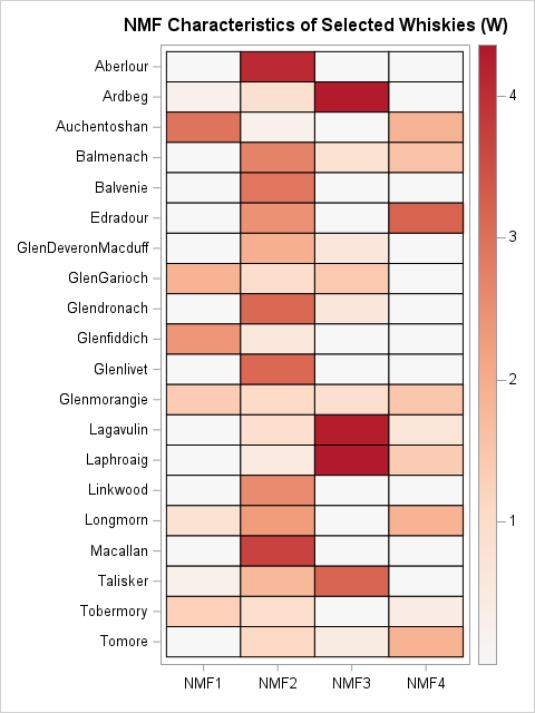
For each whisky (each row), the heat map shows the weights for the approximation of the whisky's flavor in terms of the four NMF factors. You can use this heat map in place of scatter plots to visualize the four-dimensional scores for each whisky. A few features are apparent:

The second NMF factor is used for almost all whiskies. In that sense, the second factor is a "base" set of flavors. Most individual whiskies start with this flavor profile and then add additional features by using other factors. The Aberlour, Balvenie, Glenlivet, Linkwood, and Macallan whiskies have similar flavors, which is based on the second factor. The similarity in these whiskies can be explained by noting that these distilleries are all located in the same region (Speyside) Scotland.
The first NMF factor is dominant in the Glenfiddich whisky and five others (Auchentoshan, GlenGarioch,...). Recall that the first NMF factor emphasizes "feminine" flavors such as Fruity, Sweetness, and Floral.
The third NMF factor is dominant in the Ardbeg, Lagavulin, and Laphroaig whiskies. Recall that the third NMF factor emphasizes "masculine" flavors. Indeed, all three whiskies are often described as "earthy" or "peaty," and the distilleries are all on the island of Islay.
The fourth NMF factor is primarily related to the Nutty variable. This factor is not the sole component of whisky. Rather, this factor is added to other components. The Edradour whisky is primarily composed of the "base" flavor with Nutty enhancements.

The orthogonality (not!) of NMF factors

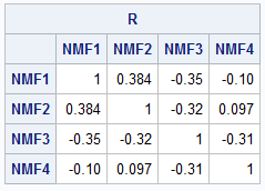
Unlike the PCA factors, the NMF factors are not orthogonal to each other. The NMF factors are correlated, as shown by the following computation:

/* show that the profile vectors are not orthogonal */
R = corr(H`);
print R[c=names r=names F=Bestd5.];

How much variance is captured by the NMF factors?

When you use a k-factor PCA for dimension-reduction, the factors form a basis for a k-dimensional linear subspace that explains the most variance in the data. Since the NMF factors are not orthogonal, the subspace spanned by the NMF factors must explain less variance. But how much less? That answer depends on the data, but you can write a short IML function that provides the answer.

The math is standard linear algebra, but a little long to explain. Let the columns of A represent a set of linearly independent basis vectors for an arbitrary subspace. To compute the variance explained by the subspace, you can project the data onto that subspace, then compute the covariance matrix of the projected data.

Let S be the covariance matrix of the original data. Briefly, you can use the following method to compute the proportion of the variance in S that is explained by the column space of A.

Let Q be an orthonormal basis for the column space of A.
The projection matrix onto this subspace is P = Q*Q`.
The covariance of the projected data is P*S*P. Therefore, the explained variance is trace(P*S*P).
The trace of a product of square matrices is invariant under a cyclic shift of the matrices in the product. If you substitute P = Q*Q`, shift the order, and simplify, you discover that the explained variance is trace(Q`*S*Q).

This method is implemented in the following SAS IML function, which accepts the covariance matrix, S, and a matrix of basis elements, A. The function returns the proportion of the variance in S that is explained by the subspace defined by the columns of A.

/* Let S be an nxn covariance matrix. 
   Let A be an nxk matrix with k linearly indep columns.
   This function returns the proportion of the variance in S that is explained by column space of A.
*/
start VarExplained(A, S);
   call svd(U, D, V, A);   /* Find orthonormal basis, Q, for the span of A */
   k = ncol(A);
   Q = U[, 1:k]; 
 
   var_explained = trace(Q`*S*Q);   /* variance explained by colspace(A) */
   total_var = trace(S);            /* total variance in S */
   prop_var = var_explained / total_var; /* proportion of var explained */
   return prop_var;
finish;
 
/* For the PCA, find the proportion of variance explained by the first 4 PCs */
call eigen(D, U, S);                 /* PCA decomp */
U = U[, 1:4];
prop_var_PCA = VarExplained(U, S);   /* somewhat redundant, since Q=U */
/* For the NMF, find the proportion of variance explained by the rowspace of H */
prop_var_NMF = VarExplained(H`, S);
print prop_var_PCA[F=PERCENT7.1] prop_var_NMF[F=PERCENT7.1];

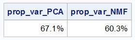
The output shows that the maximum variance that can be captured in the 4-D linear subspace is 67.1%. By comparison, the NMF factors explain 60.3% of the variance.

Summary

The purpose of this article is to use the NMF factorization on the Scotch whisky data set, which classifies the flavors in 86 Scotch whiskies according to 12 flavor characteristics. These data were analyzed by Young, Fogel, and Hawkins (2006). The NMF decomposes the data matrix into two matrices: A matrix of factors (H) and a matrix of weights (W). The NMF enables you to reduce the dimensionality of the data by replacing the 12 original variables with four factors that are nonnegative combinations of the variables. The rows of the weights matrix provides the coefficients for a rank-4 approximation of the data. The flavor profile of each whisky is approximated by using a linear combination of factors. If you visualize the weights matrix, you can identify which whiskies have similar flavor profiles.

You can download the SAS programs in this article from GitHub.

Blogs